5.05a, 5.05b - Sample means and unbiased estimates
Averages are steadier than single observations, but averaging does not turn the original population into a normal distribution. In 5.05a you will distinguish the distribution of a sample mean from the population distribution; in 5.05b you will use sample data to estimate an unknown population mean and variance without systematic bias.
The centre and spread of a sample mean
A sensor has mean reading and standard deviation . Can the mean of independent readings be six times as steady as one reading? The sensor itself does not improve. What changes is the random quantity you record: an average instead of one reading.
For example, averaging the readings , and gives . A new sample will usually give a different average. Before you take the sample, that average is a random variable in its own right.
You already know
For independent observations, expectations and variances add. Multiplying a random variable by multiplies its variance by . A normal distribution is written , with variance in the second position.
Keep the random average and its observed value separate in your notation.
Sample mean and sampling distribution
For a randomly and independently selected sample from one population, the sample mean is . Its sampling distribution describes the values of across repeated samples of that same size. After observing values , the calculated value is .
Independent fluctuations can offset one another. Averaging therefore preserves the population centre while reducing spread. The following moment results apply whether the population is normal, skewed or discrete, provided its mean and finite variance exist.
Moments of a sample mean
For independent observations from a population with mean and finite variance ,
These results hold for every positive sample size ; normality is not required.
In the formula booklet.
The standard deviation of the sampling distribution has its own useful name. Take the square root of the variance, rather than dividing the population standard deviation by .
Standard error of the mean
Under the same independent-sampling conditions,
This is the standard error of the sample mean. It is the square root of the sample-mean variance printed in the booklet, rather than a separately printed formula.
Not in the formula booklet: learn it.
Calculate the variance first if there is any risk of confusing the two denominators.
Worked example 1: averaging thirty-six readings
Question. Independent readings have population mean and variance . Find the expectation, variance and standard error of the mean of readings.
Plan. Keep the mean, divide the variance by the sample size, then take its square root.
Why this step? The spread needed is the spread of repeated averages, not the spread of individual readings.
Answer. The expectation is , the variance is , and the standard error is .
Check. . The standard error is one sixth of the individual standard deviation.
Worked example 2 changes only the sample size. Watch the difference between reducing the variance and reducing the standard error.
Worked example 2: quadrupling the sample size
Question. The same population has mean and variance . Find the expectation, variance and standard error of the mean of independent readings.
Plan. Use the new sample size in the same sampling formulae.
Why this step? Four times as many readings divide the variance by , so they divide its square root by .
Answer. The expectation is , the variance is , and the standard error is .
Check. Relative to readings, readings halve the standard error from to . Twice the precision needs four times the data.
That square-root relationship answers the opening puzzle. It also explains why taking a few extra observations gives a modest improvement rather than a dramatic one.
Watch out
Wrong: . Right: , so . Repeating one reading times does not create an independent sample and does not reduce its uncertainty.
The next calculation gives you the parameters only. Do not invent a distributional shape from them.
Exact normality and the central limit theorem
The mean and variance do not tell you the shape of a distribution. Normality needs a separate reason: either the population is normal, or a sufficiently large sample makes a normal approximation appropriate.
If individual waiting times are exponentially distributed, large samples still contain short waits and occasional long waits. The distribution of individual waits stays skewed. Repeated averages are more balanced, because a sample can combine several short waits with a long one.
[DIAGRAM: asset_name: A skew population and the distributions of its averages; asset_slug: h245_5_05_clt_means; caption: Averaging changes the distribution of the mean while the original population remains skewed; description: Three exact density curves for an exponential variable with mean 4 and the averages of 4 and 36 independent copies, all on the same horizontal scale. Their centres are all 4, their standard deviations are 4, 2 and two thirds, and the final curve has a close normal approximation drawn as a dashed line.]
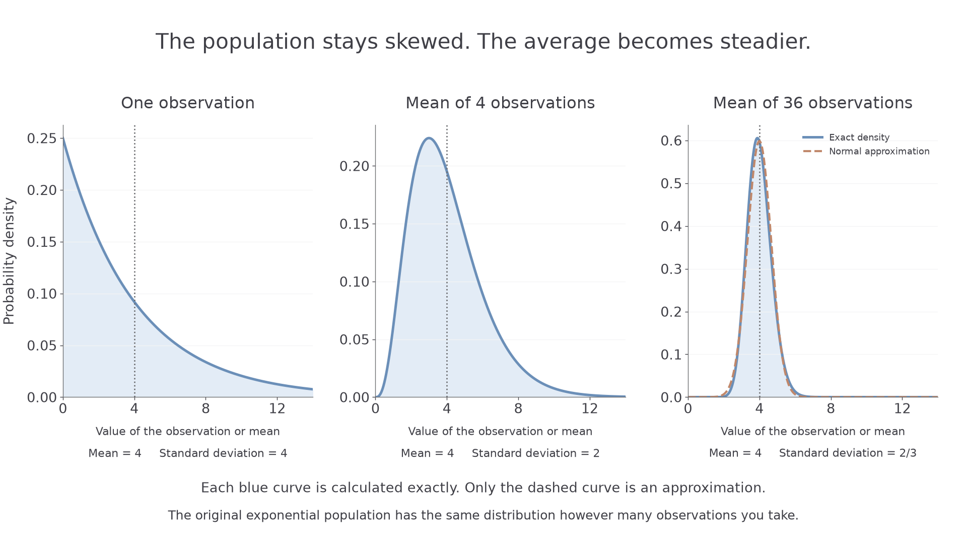
The picture shows two effects. The averages concentrate around the same centre, and their distribution becomes more nearly symmetric. Only the second effect needs the central limit theorem.
When a sample mean is normal
For a random independent sample of size :
- If , then exactly, for every .
- For any population with mean and finite positive variance , is approximately normal when is sufficiently large. Use .
The second statement is the central limit theorem. A working guide is approximately ; this is not a guarantee for every severely skewed population. The results, rather than their proofs, are required.
In the formula booklet.
State which reason you are using before calculating a probability. With a known normal population, even a small sample gives an exactly normal mean. If the population variance is zero, all observations and their average are constant; a normal approximation is unnecessary.
Worked example 3: an exactly normal average
Question. A random variable has distribution . For independent observations, find the probability that the sample mean exceeds .
Plan. Write the exact distribution of the mean and standardise the threshold.
Why this step? The standard deviation in the denominator is , the standard error, rather than , the individual standard deviation.
Answer. The probability is , to significant figures.
Check. The threshold is two standard errors above the mean, so a small upper-tail probability is sensible.
Worked example 4 changes only what is known about the population shape. The parameter calculations remain exact; the normal probability becomes an approximation.
Worked example 4: a large sample from a non-normal population
Question. A population has mean and variance , but is not normally distributed. For a random independent sample of size , estimate the probability that the sample mean exceeds .
Plan. Use the central limit theorem for the sample mean, then use its exact mean and variance in the normal approximation.
Why this step? The central limit theorem justifies the normal shape of . It does not justify the variance formula, which already holds for independent samples of every size.
Answer. The estimated probability is .
Check. The same mean, variance and sample size give the same numerical normal calculation as before. Only its exact or approximate status has changed.
Continue this lesson.
You’re previewing NovaLearn without an account. Create a free account to read the rest.
Create free account