5.07a–5.07c - Single-sample non-parametric tests
You can test a population median without fitting a normal distribution. In 5.07a you will choose an appropriate non-parametric test; in 5.07b you will see why signs and ranks provide evidence; in 5.07c you will carry out single-sample sign and Wilcoxon signed-rank tests.
Choosing signs and ranks
Nine of ten independently sampled battery lifetimes exceed a claimed median. Can that be convincing evidence even when nobody knows the shape of the lifetime distribution? A normal curve is unnecessary: under the claim, each lifetime is equally likely to fall on either side of the median.
You already know
A hypothesis concerns a population parameter. Choose the alternative and significance level before inspecting the result, then compare a tail probability with that level. Failing to reject a null hypothesis does not establish that it is true.
For a continuous population with median , half the probability lies below and half above it. The median need not equal the mean. In a strongly right-skewed distribution, a few large values can pull the mean well above the median.
Non-parametric test
A non-parametric hypothesis test does not require a specified parametric family, such as a normal distribution, for the population being investigated. It can use the signs or ranks of observations rather than their full numerical values. It still has assumptions: random sampling and independence matter, and some rank tests require symmetry.
A sign records only which side of a reference value an observation occupies. A rank records relative position. For example, the differences have one negative sign and three positive signs; the negative difference also has the largest magnitude. A sign test discards that last fact. A signed-rank test retains it.
| Data and question | Suitable test | Information used |
|---|---|---|
| One independent sample; test its median without assuming symmetry | Single-sample sign test | Counts above and below the hypothetical median |
| One independent sample from a continuous symmetric population; test its centre | Wilcoxon signed-rank test | Signs and ranks of absolute differences from the hypothetical median |
| Matched observations on the same units | Paired sign or matched-pairs signed-rank test | Within-pair differences |
| Two independent samples; compare their populations | Wilcoxon rank-sum test, also called the Mann–Whitney U test | The positions occupied by one sample in a combined ranking |
The last two rows are developed in the next lesson. Their basis is already visible: paired tests keep each genuine match; a rank-sum test instead asks whether one independent sample tends to occupy the small or large ranks in the pooled data. Under identical continuous populations, each allocation of sample labels to the pooled ranks is equally likely. A claim specifically about different medians needs populations of the same shape and spread, differing only in location.
These tests are useful for small samples whose population shape is not known to be normal. “Non-parametric” does not mean “no hypotheses”, “no parameters” or “no assumptions”. The single-sample tests here concern the population median. For the signed-rank test, symmetry is an additional assumption; the sign test does not require it.
Key idea
Choose the statistic to match both the sampling design and the assumptions you can justify. A sign needs only direction; a signed rank also uses the relative sizes of the differences.
The distinction matters before any calculation. Extra information is useful only when the assumptions needed to use it are credible.
The single-sample sign test
Count observations above the hypothetical median and use an exact binomial tail. This converts an unknown population shape into a familiar probability calculation.
Let be the population median and suppose . For independent observations from a continuous population, the indicators of exceeding are independent successes with probability . In this lesson no observation equals .
Sign-test distribution
Under , for random independent observations from a continuous population,
For , large supports the alternative; for , small does. For a two-sided alternative, use both equally extreme tails of this symmetric null distribution.
The binomial probability formula is supplied, but this sign-test model must be set up from the median property.
Not in the formula booklet: learn it.
The observed count is not itself a probability. Include outcomes at least as extreme as the one observed, in the direction of the alternative.
Worked example 1: evidence of a longer lifetime
Question. A random independent sample of battery lifetimes contains above hours and below. Test, at the significance level, whether the population median exceeds hours.
Plan. State hypotheses about the population median and find the binomial upper tail from upwards.
Why this step? The question asks whether lifetimes are longer, so or above the target supports the alternative; the lower tail does not.
Answer. Reject . There is significant evidence that the population median battery lifetime exceeds hours.
Check. Under the null, even all above the target is possible. Its probability is , which is included in the tail.
Worked example 2 changes only the alternative: a change in either direction matters. The two-sided probability therefore includes the equally extreme lower tail.
Worked example 2: evidence of a change
Question. Use the same sample to test, at the significance level, whether the population median battery lifetime differs from hours.
Plan. Keep the null distribution, replace the alternative, and combine the two symmetric tails.
Why this step? Either an unusually small or an unusually large count would now count against the null. Alternatively compare the single upper-tail probability with .
Answer. There is significant evidence that the population median battery lifetime differs from hours.
Check. The two-sided probability is twice the one-sided probability and remains below .
Here is a useful small-sample surprise: if all observations exceed a proposed median, the one-sided probability is . You can obtain evidence with six observations without claiming that six measurements reveal the population's shape.
Watch out
Wrong: . Right: for the upper-tailed test. A significance test counts the observed outcome and outcomes further in the alternative's direction, not just that single count.
The next sample changes the count by one. A modest-looking change can move a discrete tail across the significance level.
Constructing signed ranks
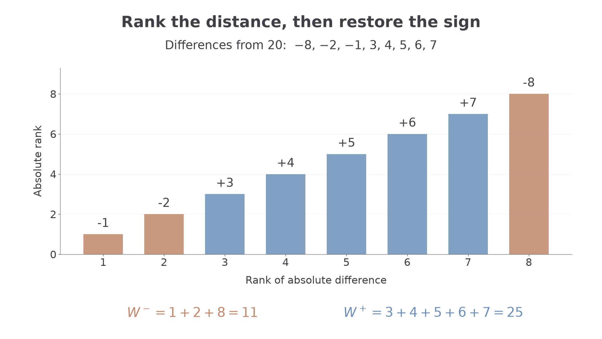
A signed-rank test distinguishes a tiny negative difference from a large negative difference. Subtract the hypothetical median first, rank the magnitudes, then return the signs.
For data , compare with . The differences are . Ranking the original data would give the negative differences ranks ; that loses the fact that the value is the furthest from .
[DIAGRAM: asset_name: Signs become signed ranks; asset_slug: h245_5_07_signed_rank_weights; caption: Rank absolute differences from the proposed median, then restore their signs; description: Eight differences from 20 shown in order of increasing magnitude, with negative differences -1, -2 and -8 coloured clay and positive differences 3, 4, 5, 6 and 7 coloured blue. Bars have heights equal to absolute ranks 1 through 8, labels show the signed differences, and the two sums are W minus equals 11 and W plus equals 25.]
Continue this lesson.
You’re previewing NovaLearn without an account. Create a free account to read the rest.
Create free account