7.07e, 7.07f - Interpreting simplex iterations | OCR A-Level Further Mathematics A

Connect a simplex iteration to movement along an edge of the feasible region, in two and three dimensions. You will explain the ratio test and row operations algebraically, then use those explanations to recognise tied optima, a degenerate step and an unbounded objective.

Iterations along polygon edges

Why does a simplex pivot move to a neighbouring vertex instead of cutting across the middle of the feasible region? Consider maximising $P = 3x + 2y$ , subject to $x+y\le9$ , $2x+y\le12$ and $x,y\ge0$ . The first two iterations follow $O=(0,0)$ , $A=(6,0)$ , $B=(3,6)$ . We will identify exactly which boundary each move follows.

You already know

A slack equation, such as $2x+y+t=12$ , makes $t=0$ equivalent to using that resource completely. In a tableau, set non-basic variables to zero and read the basic variables from their unit columns.

The feasible set is a convex polygon: the whole line segment joining any two feasible points is feasible. For a linear inequality this follows by taking the same weighted average of the two inequalities. Intersecting several such half-planes preserves this property.

Convex feasible region

A region is convex if the segment joining any two points in the region lies entirely inside it. A bounded three-dimensional region cut out by linear inequalities is a convex polyhedron; the corresponding object in any number of dimensions is a convex polytope. A polygon is the two-dimensional case.

With two decision variables, a non-degenerate vertex normally lies on two active boundaries. During an ordinary pivot, one of these remains active: its variable or slack stays zero. The entering variable increases until a different boundary is reached. This is movement along an edge, rather than through the interior.

[DIAGRAM: asset_name: Two simplex iterations follow boundary edges; asset_slug: h245_7_07_simplex_polygon; caption: The first move follows y = 0 from O to A; the second follows t = 0, or 2x + y = 12, from A to B; description: Equal-scale axes show the feasible quadrilateral with vertices O=(0,0), A=(6,0), B=(3,6), C=(0,9). Excluded half-planes beyond x+y=9 and 2x+y=12 are pale shaded, leaving the polygon white. A blue arrow follows O to A on y=0, and a clay arrow follows A to B on 2x+y=12. Labels show objective values 0,18,21 at O,A,B and label both constraint boundaries without overlap]
The first move follows y = 0 from O to A

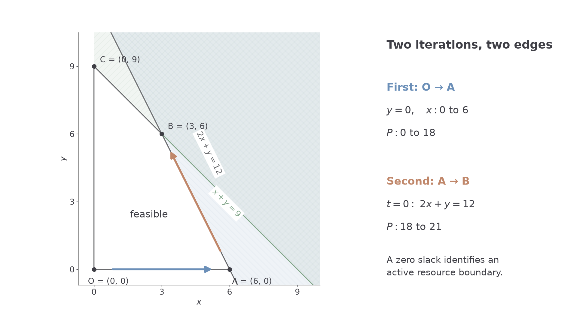
The two examples distinguish the first edge from the second. “The edge” must refer to the iteration actually named in the question.

Worked example 1: interpreting the first iteration

Question. For the opening problem, interpret the first simplex iteration geometrically. State its beginning and end vertices and the edge followed.

Plan. Read the initial basic solution, identify the first entering variable and keep the other non-basic variable zero.

\begin{aligned} x=y=0 &\Rightarrow (x,y)=(0,0) && \text{initial vertex}\\ -3<-2 &\Rightarrow x\text{ enters} && \text{most negative objective entry}\\ x&\le\min\{9,12/2\}=6 && \text{ratio bounds with }y=0\\ x=6,\ y=0 &\Rightarrow s=3,\ t=0 && \text{end vertex} \end{aligned}

Why this step? The variable $y$ is non-basic before and after this iteration, so it stays zero along the whole move.

Answer. Move from $O=(0,0)$ to $A=(6,0)$ along the edge $y=0$ , with $0\le x\le6$ .

Check. Along that segment both resource inequalities hold. The objective increases from $0$ to $18$ .

The second example changes only which iteration is being interpreted. The new edge is no longer an axis.

Worked example 2: interpreting the second iteration

Question. After the first iteration, the opening problem has tableau

\begin{array}{c|rrrrr|r} &P&x&y&s&t&\mathrm{RHS}\\ \hline &1&0&-\frac12&0&\frac32&18\\ &0&0&\frac12&1&-\frac12&3\\ &0&1&\frac12&0&\frac12&6 \end{array}

Interpret the second iteration geometrically.

Plan. Keep the non-basic variable that does not enter equal to zero, then use the ratio test to locate the next vertex.

\begin{aligned} y&\text{ enters},\qquad t=0 && \text{negative objective entry}\\ y&\le\min\{3/(1/2),6/(1/2)\}=6 && \text{ratio test}\\ y=6&\Rightarrow s=0,\quad x=3 && \text{end of the edge}\\ t=0&\iff 2x+y=12 && \text{active resource boundary} \end{aligned}

Why this step? The common zero variable is $t$ , not $y$ : $y$ is now the variable increasing along the edge.

Answer. Move from $A=(6,0)$ to $B=(3,6)$ along $t=0$ , or $2x+y=12$ .

Check. Both endpoints satisfy $2x+y=12$ ; their objective values are $18$ and $21$ . At $B$ , $x+y=9$ , so the next boundary has been reached.

These geometric interpretations and the convexity argument are not in the formula booklet: learn them.

Watch out

Wrong: identify the edge from variables that are zero at only one endpoint. Right: find the boundary that remains active throughout the move, using the zero variable shared by the beginning and end vertices.

For the next move, distinguish the resource boundary from the coordinate axis.

Iterations along polyhedron edges

With three decision variables, a single active plane gives a face; an edge normally needs two active planes.

Consider the non-negative variables $x,y,z$ , with

x+y+z+s=6,\qquad 2x+y+z+t=8,\qquad y+2z+u=6

where $s,t,u\ge0$ . A vertex normally has three independent active boundaries. During a non-degenerate pivot, two remain active, defining the edge of the polyhedron.

A useful way to identify that edge is to list the decision and slack variables that are zero at both endpoints. Translate their zero values into plane equations when necessary. The objective variable is not one of the coordinates.

[DIAGRAM: asset_name: Different objectives select different edges of a polyhedron; asset_slug: h245_7_07_simplex_polyhedron; caption: From A, y entering follows z = t = 0 towards B; z entering instead follows y = t = 0 towards C; description: A three-dimensional exact feasible polyhedron is shown for non-negative x,y,z with x+y+z<=6, 2x+y+z<=8, y+2z<=6. Pale faces and thin grey edges reveal its shape. A=(4,0,0), B=(2,4,0) and C=(5/2,0,3) are marked. A clay arrow traces A to B in the z=0 face, and a blue arrow traces A to C in the y=0 face. Separate annotations identify the shared plane 2x+y+z=8 and the two pairs of zero variables. Axes are labelled x,y,z and the origin O is marked]
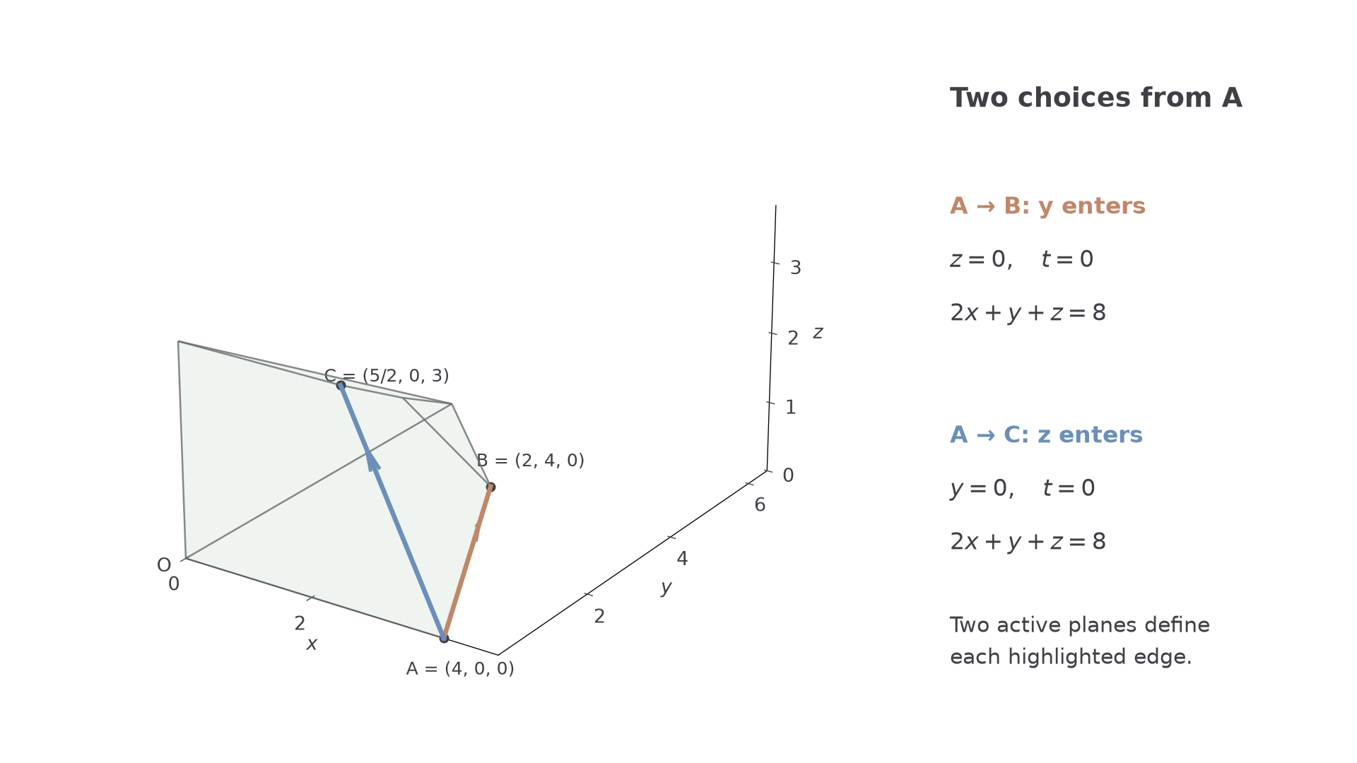
From A, y entering follows z = t = 0 towards B

The objective selects which available edge to follow. The following pair changes just one profit coefficient.

Worked example 3: an edge defined by two zero variables

Question. Maximise $P=4x+3y+2z$ subject to the three constraints above. After the first iteration the tableau is

\begin{array}{c|rrrrrrr|r} &P&x&y&z&s&t&u&\mathrm{RHS}\\ \hline &1&0&-1&0&0&2&0&16\\ &0&0&\frac12&\frac12&1&-\frac12&0&2\\ &0&1&\frac12&\frac12&0&\frac12&0&4\\ &0&0&1&2&0&0&1&6 \end{array}

Interpret the next iteration geometrically.

Plan. Read its starting vertex, choose the entering column and identify the non-basic variables that remain zero.

\begin{aligned} y=z=t=0 &\Rightarrow (x,y,z)=(4,0,0) && \text{starting vertex}\\ y&\text{ enters} && \text{only negative objective entry}\\ y&\le\min\{2/(1/2),4/(1/2),6/1\}=4 && \text{ratio bounds}\\ y=4 &\Rightarrow (x,y,z)=(2,4,0) && \text{read the constraint equations} \end{aligned}

Why this step? The non-basic variables $z$ and $t$ remain zero; their two planes define the edge.

Answer. Move from $A=(4,0,0)$ to $B=(2,4,0)$ along the edge

z=0,\qquad t=0

or, equivalently, $z=0$ and $2x+y+z=8$ .

Check. At $A$ , $(s,t,u)=(2,0,6)$ ; at $B$ , $(s,t,u)=(0,0,2)$ . The objective increases from $16$ to $20$ .

The next example changes only the coefficient of $z$ from $2$ to $7/2$ . The constraints and first vertex $A$ remain unchanged, but the next entering column changes.

Worked example 4: another edge from the same vertex

Question. Change the objective to $P=4x+3y+\frac72z$ . After the first iteration the constraint rows are unchanged, but the objective row is

P-y-\tfrac32z+2t=16

Interpret the next iteration.

Plan. Choose the more negative objective coefficient and apply the ratio test in that column.

\begin{aligned} -\tfrac32&<-1 && z\text{ enters}\\ z&\le\min\{2/(1/2),4/(1/2),6/2\}=3 && \text{positive column entries}\\ y=t=0,\ z=3 &\Rightarrow x=4-\tfrac12(3)=\tfrac52 && \text{read the }x\text{ row}\\ u&=6-2(3)=0,\qquad s=2-\tfrac12(3)=\tfrac12 && \text{remaining slacks} \end{aligned}

Why this step? Here $y$ , rather than $z$ , stays non-basic; the move therefore follows a different edge of the same feasible region.

Answer. Move from $A=(4,0,0)$ to $C=(5/2,0,3)$ , along $y=t=0$ . Equivalently, the two planes are $y=0$ and $2x+y+z=8$ .

Check. At $C$ , the original constraint totals are $11/2\le6$ , $8\le8$ , $6\le6$ . The new objective rises from $16$ to $41/2$ .

The geometric interpretation in three dimensions is not in the formula booklet. At a degenerate vertex, more boundaries can be active and a pivot need not move to a different point; the ordinary two-plane description above assumes a non-degenerate edge move.

Continue this lesson.

You’re previewing NovaLearn without an account. Create a free account to read the rest.

Create free account

Last Accessed

Pure Core

Statistics

Mechanics

Discrete Mathematics

Additional Pure Mathematics

7.07e, 7.07f - Interpreting simplex iterations

Iterations along polygon edges

Iterations along polyhedron edges

Continue this lesson.

Learn faster with Nova