5.03e–5.03g - Cumulative distribution functions | OCR A-Level Further Mathematics A

A cumulative distribution function stores every left-tail probability in one curve. In 5.03e–5.03f you will construct and use that curve, recover its density and locate percentiles; 5.03g then uses inequalities to find the distributions of related variables.

Constructing a c.d.f.

If you choose a random value $X$ from a continuous distribution and report the fraction of the distribution lying below it, what distribution does that reported fraction have? For a steadily increasing cumulative curve, the answer is unexpectedly simple: it spreads uniformly between $0$ and $1$ . You will see one exact example by the end of the lesson.

You already know

A density $f$ is non-negative with total area $1$ , and $\mathrm{P}(a<X<b)=\int_a^b f(x)\,dx$ . Individual points have probability zero, so strict and inclusive endpoints give the same probability.

Start with the density $f(x)=\frac{x}{2}$ on $[0,2]$ . The area to the left of $1$ is $\int_0^1\frac{x}{2}\,dx=\frac14$ ; the area to the left of $2$ is $1$ . Letting the endpoint move turns these separate answers into a function.

Cumulative distribution function

The cumulative distribution function, or c.d.f., of $X$ is

F(x)=\mathrm{P}(X\le x)

It gives the total probability at or to the left of $x$ . For a continuous variable it is continuous, never decreases, and has limiting values $0$ and $1$ at the far left and far right. It can have flat intervals when the density is zero there.

A density describes probability per unit width; its c.d.f. describes accumulated probability. Use a different letter inside the integral so that the endpoint $x$ is not confused with the variable being integrated.

Cumulative probability

For a continuous variable with p.d.f. $f$ ,

F(x)=\mathrm{P}(X\le x)=\int_{-\infty}^{x}f(t)\,dt

In the formula booklet.

The limits outside a finite support are part of the answer: no area has accumulated before the support, and all the area has accumulated after it.

Worked example 1: the whole real line

Question. Find the c.d.f. of $X$ with density $f(x)=\frac{x}{2}$ for $0\le x\le2$ , and zero otherwise.

Plan. Find the integral within the support, then include the constant branches outside it.

\begin{aligned} F(x)&=\int_0^x\frac{t}{2}\,dt=\frac{x^2}{4} &&0\le x\le2\\ F(0)&=0,\qquad F(2)=1 &&\text{check the joins} \end{aligned}

Why this step? $F$ is a probability for every real input, including inputs outside the support of $X$ .

Answer.

F(x)=\begin{cases}0&x<0\\\frac{x^2}{4}&0\le x\le2\\1&x>2\end{cases}

Check. $F(1)=\frac14$ , agreeing with the area calculated above; $F$ rises continuously from $0$ to $1$ .

Worked example 2 changes one feature: the density is piecewise. The second branch of the c.d.f. must retain all the probability accumulated in the first branch.

Worked example 2: carrying area across a join

Question. Find the c.d.f. when $f(x)=x$ for $0\le x\le1$ , $f(x)=2-x$ for $1<x\le2$ , and zero otherwise.

Plan. Integrate from $0$ on the first interval; on the second, add the area already accumulated up to $1$ .

\begin{aligned} F(x)&=\int_0^x t\,dt=\frac{x^2}{2} &&0\le x\le1\\ F(x)&=\frac12+\int_1^x(2-t)\,dt &&1<x\le2\\ &=\frac12+2x-\frac{x^2}{2}-\frac32 &&\text{insert the lower limit}\\ &=1-\frac{(2-x)^2}{2} &&\text{simplify} \end{aligned}

Why this step? Restarting the second integral at zero probability would throw away the first half of the distribution.

Answer.

F(x)=\begin{cases}0&x<0\\\frac{x^2}{2}&0\le x\le1\\1-\frac{(2-x)^2}{2}&1<x\le2\\1&x>2\end{cases}

Check. Both middle expressions give $F(1)=\frac12$ , and the second gives $F(2)=1$ . The c.d.f. is continuous at every join.

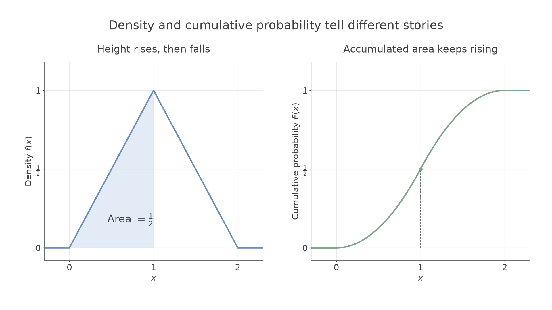
The density rises and then falls, but the c.d.f. keeps rising: positive density always adds probability.

[DIAGRAM: asset_name: A density and its accumulated area; asset_slug: h245_5_03_density_cdf; caption: The triangular density rises then falls, while its cumulative distribution function always rises and reaches one; description: Two separate labelled panels show the triangular density x then 2 minus x on 0 to 2, and its c.d.f. x squared over 2 then 1 minus half of 2 minus x squared. Dashed guides mark x equals 1 and cumulative probability one half; the c.d.f. is zero before 0 and one after 2]
The triangular density rises then falls, while its cumulative distribution function always rises and reaches one

Watch out

Wrong on the second interval: $F(x)=\int_1^x(2-t)\,dt$ , giving $F(1)=0$ . Right: add $F(1)=\frac12$ . A continuous variable's c.d.f. cannot jump at the join.

Use the outside branches and continuity as quick checks before calculating anything from your c.d.f.

Using and differentiating a c.d.f.

Once cumulative probabilities are available, an interval probability is a subtraction and the density is the slope.

From c.d.f. to probabilities and density

For a continuous variable,

\begin{aligned} \mathrm{P}(a<X\le b)&=F(b)-F(a)\\ \mathrm{P}(X>x)&=1-F(x)\\ f(x)&=F'(x)\quad\text{where }F\text{ is differentiable} \end{aligned}

The derivative relation follows from the c.d.f. integral in the booklet. These rules are not printed there separately.
Not in the formula booklet: learn it.

At a corner of $F$ , a derivative need not exist. The value assigned to the density at an individual point does not affect any probability. What matters is the slope on each open interval and the correct support.

Worked example 3: recover the density and an interval

Question. A continuous variable has c.d.f.

F(x)=\begin{cases}0&x<0\\\frac{x^3}{8}&0\le x\le2\\1&x>2\end{cases}

Find its density and $\mathrm{P}(\frac12<X<\frac32)$ .

Plan. Differentiate the non-constant branch and subtract the two cumulative probabilities.

\begin{aligned} f(x)&=\frac{3x^2}{8} &&0<x<2\\ \mathrm{P}\left(\frac12<X<\frac32\right)&=F\left(\frac32\right)-F\left(\frac12\right) &&\text{remove the lower tail}\\ &=\frac{27}{64}-\frac1{64}=\frac{13}{32} &&\text{insert both endpoints} \end{aligned}

Why this step? $F(\frac32)$ includes all values below $\frac12$ , which the requested event excludes.

Answer. $f(x)=\frac{3x^2}{8}$ for $0<x<2$ , and zero outside the support; the probability is $\frac{13}{32}$ . Endpoint density values may be chosen without changing the distribution.

Check. $\int_0^2\frac{3x^2}{8}\,dx=1$ , and integrating it directly from $\frac12$ to $\frac32$ gives $\frac{13}{32}$ .

Worked example 4 changes one feature: the distribution is reflected about $1$ . The interval stays the same, so the probability should be unchanged even though the density slopes the other way.

Worked example 4: a decreasing density

Question. A continuous variable has c.d.f.

G(x)=\begin{cases}0&x<0\\1-\frac{(2-x)^3}{8}&0\le x\le2\\1&x>2\end{cases}

Find its density and $\mathrm{P}(\frac12<X<\frac32)$ .

Plan. Differentiate carefully using the chain rule, then subtract cumulative values.

\begin{aligned} g(x)&=-\frac38(2-x)^2(-1)=\frac{3(2-x)^2}{8} &&0<x<2\\ \mathrm{P}\left(\frac12<X<\frac32\right)&=\left(1-\frac1{64}\right)-\left(1-\frac{27}{64}\right) &&G(b)-G(a)\\ &=\frac{13}{32} &&\text{simplify} \end{aligned}

Why this step? The chain-rule factor $-1$ makes the derivative positive, as every density must be.

Answer. $g(x)=\frac{3(2-x)^2}{8}$ for $0<x<2$ , zero outside; the probability is $\frac{13}{32}$ .

Check. The reflected interval is the same interval, so reflection preserves its probability. Also $G$ increases from $0$ to $1$ , although $g$ decreases.

If $F(a)>0$ , conditional probabilities such as $\mathrm{P}(X\le b\mid X\le a)$ , with $b<a$ , become $F(b)/F(a)$ . First identify the intersection, as with any conditional event.

Watch out

Wrong: $\mathrm{P}(X>x)=F(x)$ . The c.d.f. is the left tail. Right: $\mathrm{P}(X>x)=1-F(x)$ . Likewise, differentiating $F$ gives the density, not another probability.

For piecewise c.d.f.s, differentiate each branch separately and choose the correct branch at each probability endpoint.

Median, quartiles and percentiles

A percentile reverses a cumulative-probability calculation: the probability is known, and the boundary is unknown.

Percentiles

A percentile $q$ at cumulative probability $p$ satisfies $F(q)=p$ , where $0<p<1$ . The median uses $p=\frac12$ , and the lower and upper quartiles use $p=\frac14$ and $p=\frac34$ . For example, the ninetieth percentile leaves probability $0.9$ to its left and $0.1$ to its right. If $F$ is flat at the required level, more than one boundary can satisfy the equation; use the problem's stated convention if it asks for a unique choice.

Choose the correct branch before solving. For the triangular distribution above, $F(1)=\frac12$ , so its lower quartile lies below $1$ and its upper quartile lies above it.

Percentile equation

For a continuous distribution, find the percentile at cumulative probability $p$ by solving

F(q)=p

with $q$ in the support and in the interval for the branch used. Equivalently, solve $\int_{-\infty}^{q}f(x)\,dx=p$ .
Not in the formula booklet: learn it.

A square root or logarithm may produce algebraic candidates. A candidate outside its branch interval is not a percentile of that branch.

Worked example 5: the lower quartile

Question. For the triangular density $f(x)=x$ on $[0,1]$ and $f(x)=2-x$ on $(1,2]$ , find the lower quartile.

Plan. Use $F(q)=\frac14$ ; the quartile lies in the first branch because $F(1)=\frac12$ .

\begin{aligned} \frac{q^2}{2}&=\frac14 &&\text{first c.d.f. branch}\\ q^2&=\frac12 &&\text{rearrange}\\ q&=\frac1{\sqrt2} &&0\le q\le1 \end{aligned}

Why this step? The negative square root solves the algebraic equation but lies outside the support.

Answer. The lower quartile is $\frac1{\sqrt2}$ .

Check. It is between $0$ and $1$ , and $F(\frac1{\sqrt2})=\frac12(\frac12)=\frac14$ .

Continue this lesson.

You’re previewing NovaLearn without an account. Create a free account to read the rest.

Create free account

Last Accessed

Pure Core

Statistics

Mechanics

Discrete Mathematics

Additional Pure Mathematics

5.03e–5.03g - Cumulative distribution functions

Constructing a c.d.f.

Using and differentiating a c.d.f.

Median, quartiles and percentiles

Continue this lesson.

Learn faster with Nova