5.06d - Chi-squared goodness of fit tests
Use expected frequencies to test whether a proposed probability distribution is compatible with observed data. You will combine adjacent classes, allow for parameters estimated from the sample, choose a critical value and give a conclusion that distinguishes lack of evidence from proof of a model.
Testing given proportions
Can the same observed and expected frequency tables lead to different goodness of fit decisions? They can, when the hypotheses used different amounts of information from the sample. We will first test a fully specified model, then see why estimating a parameter changes the comparison.
You already know
For a proposed model, . Continuous class probabilities are areas or c.d.f. differences; unbounded models need a final tail class. An independence test compares two categorical variables, while a goodness of fit test compares one observed distribution with a proposed model.
The null hypothesis states the proposed population distribution. The alternative says it does not have that distribution. For example, : category probabilities are in the ratio ; : they are not in that ratio. Do not put “there is evidence” into the hypotheses: evidence is what the test will assess.
Goodness of fit statistic
For mutually exclusive, exhaustive classes with expected frequencies ,
Under the null hypothesis, this is approximately distributed as , with appropriate degrees of freedom.
In the formula booklet.
For retained classes and a fully specified model, , because the frequencies sum to the fixed total . This degrees-of-freedom rule is not printed in the booklet. Large discrepancies give large statistics, so use an upper-tail critical value. The critical-value table is in the formula booklet.
Worked example 1: a fully specified ratio
Question. A random sample of independent observations has category frequencies . Test at the level whether the population proportions are in the ratio .
Plan. State the ratio hypotheses, find expected frequencies, calculate the statistic and use degrees of freedom.
: population proportions are . : they are not .
Why this step? The ratio is specified before using the sample; no parameter has been adjusted to make the model fit better.
Answer. Do not reject . There is insufficient evidence at the level that the population proportions differ from .
Check. Expected frequencies sum to and all exceed ; the contributions are approximately .
Worked example 2 changes only the observed allocation between the first two categories. Keep the hypothesis, expected frequencies and critical value fixed.
Worked example 2: a larger discrepancy
Question. For the same proposed ratio, another random sample of independent observations has frequencies . Carry out the goodness of fit test.
Plan. Use the same expected table and calculate the new contributions.
The hypotheses remain : population proportions are ; : they are not.
Why this step? Squaring the larger first-category discrepancy increases its contribution from to .
Answer. Reject . There is sufficient evidence at the level that the population proportions differ from .
Check. The first contribution is , so the full statistic must already exceed .
A goodness of fit test does not use Yates’s correction, even with only two retained classes or one degree of freedom. In this course that correction belongs to a two-by-two contingency table for independence.
Exam tip
Give the statistic, retained degrees of freedom, critical value and numerical comparison before the conclusion. A non-significant result needs “insufficient evidence that the model does not fit”, or equivalent qualified wording, rather than “the model is correct”.
Keep the conclusion attached to the population proportions the question actually proposed.
Pooling adjacent classes
Pool adjacent classes until every expected frequency in the retained table is at least , then calculate both the statistic and degrees of freedom from that table.
Add the observed frequencies and the expected frequencies separately. In particular,
is the pooled contribution; adding the old individual contributions is generally different. This expression follows from the booklet's statistic and is not separately printed there. Decide pooling from expected sizes, without choosing groups to obtain a preferred test outcome.
Worked example 3: merge a small upper tail
Question. A fixed model is proposed for independent trial counts. For classes , the observed frequencies are . Carry out a goodness of fit test.
Plan. Include the infinite tail, combine its small adjacent classes, then test the retained table.
: trial counts have distribution . : they do not.
The retained classes are , with observed frequencies and expectations .
Why this step? Combining only the last two classes gives expectation , still too small. The tail must begin at here.
Answer. Do not reject . There is insufficient evidence at the level that these trial counts do not follow the specified geometric distribution.
Check. Both retained tables sum to , and the smallest retained expectation is .
Worked example 4 changes only the sample size to , with another set of observed counts. Halving the model expectations forces the tail to begin one class earlier.
Worked example 4: a smaller sample needs more pooling
Question. For the same fixed model, independent observations give frequencies in the same original classes. Carry out a test.
Plan. Recalculate expectations for , then find the smallest suitable upper-tail group.
The hypotheses remain the same fixed geometric model and its negation.
Why this step? The original class boundaries are not sacred: the expected-frequency requirement determines the retained boundaries before the statistic is formed.
Answer. Do not reject . There is insufficient evidence at the level against the specified geometric model for these trial counts.
Check. Retained expectations and observations both sum to .
[DIAGRAM: asset_name: Pooling changes the number of retained classes; asset_slug: h245_5_06_pooling_geometric_tail; caption: With 80 observations the retained tail starts at 5, while with 40 it must start at 4; description: Two rows of class boxes show geometric expected frequencies for success probability one half. The upper row for sample size 80 shows 40, 20, 10, 5, 2.5, 1.25, 1.25 in classes 1, 2, 3, 4, 5, 6, at least 7. The final three combine into a tail of expected size 5. The lower row for sample size 40 shows 20, 10, 5, 2.5, 1.25, 0.625, 0.625. The final four combine into a tail of expected size 5. The resulting retained class counts are five and four respectively]
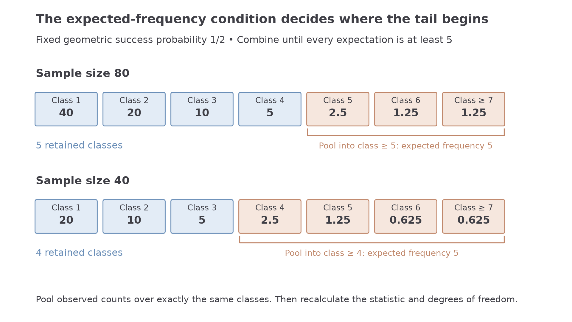
Pooling applies equally to continuous intervals: adjacent intervals become their union, and an open final tail remains included. If pooling leaves too few classes for positive degrees of freedom, the proposed chi-squared procedure cannot be used.
Watch out
Wrong: pool because an observed frequency is below , then keep the old degrees of freedom. Right: pool because an expected frequency is below , and count the classes after pooling.
Recheck the sum of expectations and the smallest expectation before moving to the critical-value table.
Continue this lesson.
You’re previewing NovaLearn without an account. Create a free account to read the rest.
Create free account