7.06e, 7.06f - Changing coefficients and integer programming | OCR A-Level Further Mathematics A

Find when a changed coefficient preserves an optimum and when it changes the answer. Then use continuous relaxations, bounds and branching to prove an integer optimum, including problems where nearby rounded points are not enough.

Changing objective coefficients

How much can an item's profit change before a production plan stops being best? An optimum is often stable over a whole interval of prices. The key is to compare the current vertex with the vertices that could replace it.

You already know

A linear objective over a bounded feasible polygon attains an optimum at a vertex. Its level lines are parallel; equal objective values at adjacent optimal vertices make the whole joining edge optimal. Integer solutions must also have integer coordinates.

Use the region $x, y \ge 0$ , $x + y \le 6$ , $x + 2y \le 8$ . Its vertices are $(0, 0)$ , $A = (6, 0)$ , $B = (4, 2)$ and $C = (0, 4)$ . Maximising $P = ax + by$ , with $a, b > 0$ , gives the vertex values $0$ , $6a$ , $4a + 2b$ and $4b$ .

For $B$ to remain optimal, it must be at least as good as both neighbours:

\begin{aligned} 4a + 2b &\ge 6a \quad\Rightarrow\quad b \ge a && \text{compare with } A \\ 4a + 2b &\ge 4b \quad\Rightarrow\quad b \le 2a && \text{compare with } C \end{aligned}

Thus $a \le b \le 2a$ . Strict inequalities give a unique optimum at $B$ . At $b = a$ , edge $AB$ is optimal; at $b = 2a$ , edge $BC$ is optimal. These comparison and gradient criteria are not in the formula booklet: learn them.

Worked example 1: one variable profit coefficient

Question. Over this region, maximise $P = 3x + by$ , where $b > 0$ . Determine the values of $b$ for which $(4, 2)$ is optimal, and state when it is the unique optimum.

Plan. Compare $P(4, 2)$ with the objective at the other vertices.

\begin{aligned} P(4, 2) &= 12 + 2b && \text{current vertex} \\ 12 + 2b &\ge 18 \quad\Rightarrow\quad b \ge 3 && \text{compare with } (6, 0) \\ 12 + 2b &\ge 4b \quad\Rightarrow\quad b \le 6 && \text{compare with } (0, 4) \end{aligned}

The origin gives $0$ , which is smaller because $b > 0$ .

Why this step? An interval needs both comparisons: checking only one neighbour misses the point where the other becomes better.

Answer. $(4, 2)$ is optimal for $3 \le b \le 6$ , and uniquely optimal for $3 < b < 6$ . At $b = 3$ , every point on $AB$ is optimal; at $b = 6$ , every point on $BC$ is optimal.

Check. For $b = 4$ , the values at $A, B, C$ are $18, 20, 16$ . For $b = 7$ , they are $18, 26, 28$ , so $C$ has replaced $B$ .

The next example changes both coefficients together. A single parameter now rotates the objective line by increasing one contribution while decreasing the other.

Worked example 2: two linked coefficient changes

Question. Maximise $P = (3 + t)x + (4 - t)y$ over the same region. Determine the range of $t$ for which $(4, 2)$ is optimal.

Plan. Compare its objective with the values at $A$ , $C$ and the origin.

\begin{aligned} P(B) &= 4(3 + t) + 2(4 - t) = 20 + 2t && \text{substitute } B \\ P(A) &= 18 + 6t,\quad P(C) = 16 - 4t && \text{other non-zero vertices} \\ 20 + 2t &\ge 18 + 6t \quad\Rightarrow\quad t \le \frac12 && \text{beat or tie } A \\ 20 + 2t &\ge 16 - 4t \quad\Rightarrow\quad t \ge -\frac23 && \text{beat or tie } C \end{aligned}

On this interval $20 + 2t > 0$ , so the origin is also beaten.

Why this step? Direct vertex comparisons remain safe even when the parameter could make a coefficient negative outside the eventual interval.

Answer. $-\frac23 \le t \le \frac12$ . The optimum is unique in the open interval. At the lower endpoint $BC$ is optimal; at the upper endpoint $AB$ is optimal.

Check. At $t = 1/2$ , $P(A) = P(B) = 21$ . At $t = -2/3$ , $P(B) = P(C) = 56/3$ .

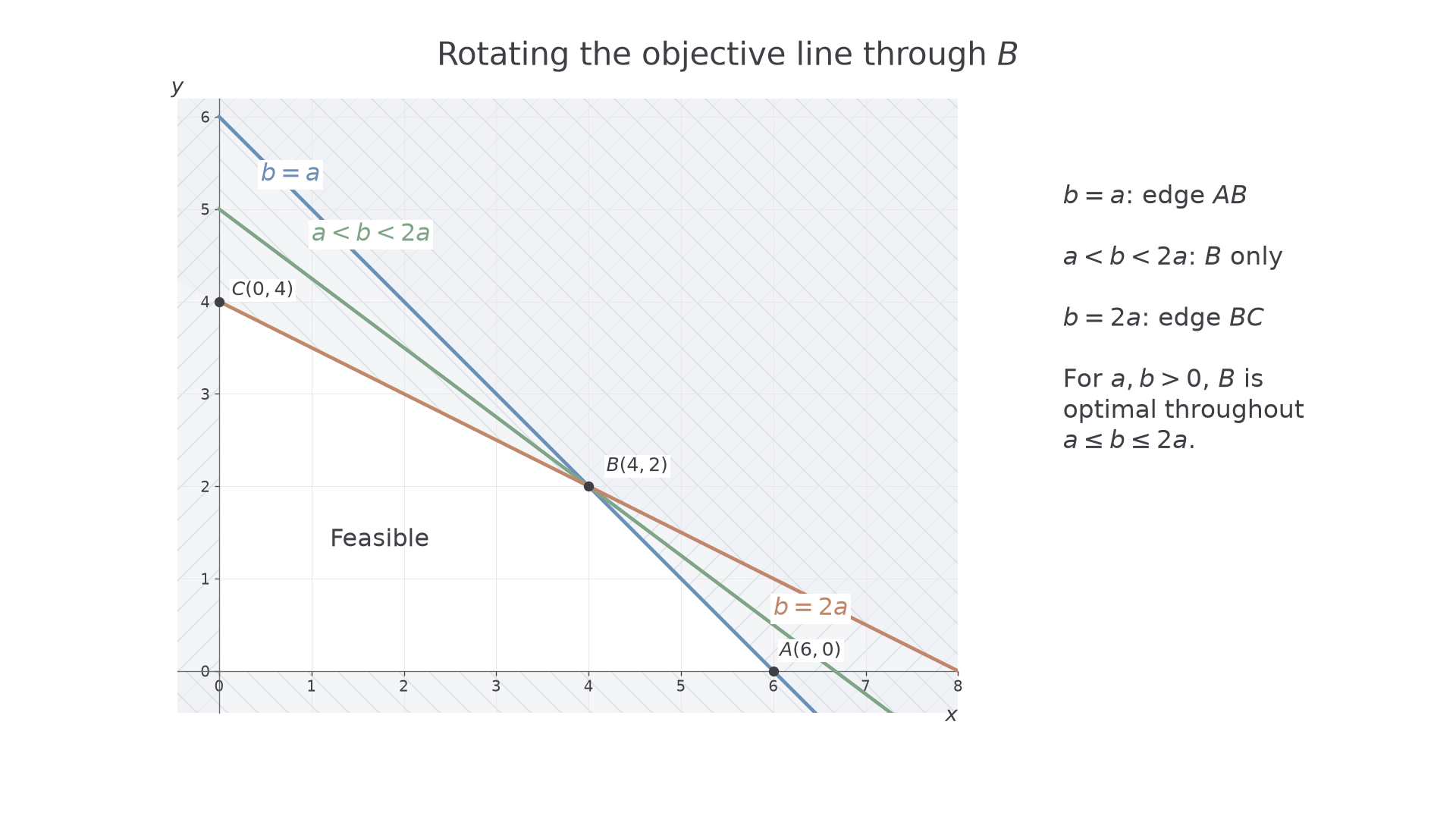
The same result can be seen by rotating the objective line: its gradient must lie between those of the two incident boundary edges.

[DIAGRAM: asset_name: A range of objective gradients selects the same vertex; asset_slug: h245_7_06_coefficient_range; caption: The vertex B remains optimal while a <= b <= 2a; equality makes a neighbouring edge optimal; description: Equal-scale axes show the feasible quadrilateral with excluded regions shaded and vertices A(6,0), B(4,2), C(0,4), O. Three objective lines through B have gradients -1, -3/4 and -1/2. The limiting lines coincide with edges AB and BC; the middle line touches only B. A side panel states b = a gives edge AB, a < b < 2a gives B only, b = 2a gives edge BC]
The vertex B remains optimal while a <= b <= 2a

Watch out

Wrong: replace $3 \le b \le 6$ by $3 < b < 6$ when asked when $B$ is optimal. The endpoints still make $B$ optimal; they only remove uniqueness. Keep “optimal” and “uniquely optimal” separate.

Now compare the same vertex under a different fixed coefficient.

Changing constraint coefficients

Changing a resource coefficient changes the feasible region itself, so an old vertex cannot simply be reused.

For example, changing $x + y \le 6$ to $2x + y \le 6$ means that each unit of $x$ uses twice as much of that resource. The vertical intercept stays at $6$ , while the horizontal intercept moves from $6$ to $3$ . Redraw the affected boundary, find the new surviving vertices and then optimise the objective. A change to the right-hand side would instead translate this boundary parallel to itself; in either case, recheck feasibility.

Worked example 3: a resource coefficient doubles

Question. Maximise $P = 3x + 4y$ , subject to $2x + y \le 6$ , $x + 2y \le 8$ and $x, y \ge 0$ .

Plan. Recalculate the intersection after the coefficient change and compare every new vertex.

\begin{aligned} 2x + y &= 6,\quad x + 2y = 8 && \text{new boundaries} \\ 3x &= 4 \quad\Rightarrow\quad x = \frac43 && \text{eliminate } y \\ y &= \frac{10}{3} && \text{substitute back} \\ P &= 3\left(\frac43\right) + 4\left(\frac{10}{3}\right) = \frac{52}{3} && \text{objective at the intersection} \end{aligned}

The other vertices $(0, 0)$ , $(3, 0)$ and $(0, 4)$ give $0$ , $9$ and $16$ .

Why this step? The old optimum $(4, 2)$ uses $2(4) + 2 = 10 > 6$ , so it is no longer feasible.

Answer. The new maximum is $52/3$ , at $(4/3, 10/3)$ .

Check. $2(4/3) + 10/3 = 6$ and $4/3 + 2(10/3) = 8$ .

The next example changes only that coefficient again, from $2$ to $3$ . The method stays the same even though the intersection moves.

Worked example 4: a further resource change

Question. Maximise $P = 3x + 4y$ , subject to $3x + y \le 6$ , $x + 2y \le 8$ and $x, y \ge 0$ .

Plan. Find the new intersection and check it against the axis vertices.

\begin{aligned} 3x + y &= 6,\quad x + 2y = 8 && \text{active boundaries} \\ 5x &= 4 \quad\Rightarrow\quad x = \frac45 && \text{eliminate } y \\ y &= \frac{18}{5} && \text{substitute} \\ P &= \frac{12}{5} + \frac{72}{5} = \frac{84}{5} && \text{evaluate} \end{aligned}

The other vertices $(0, 0)$ , $(2, 0)$ and $(0, 4)$ give $0$ , $6$ and $16$ , all smaller than $84/5$ .

Why this step? An intersection is a candidate, not automatically the answer; comparing the remaining vertices establishes the maximum.

Answer. The maximum is $84/5$ , at $(4/5, 18/5)$ .

Check. $3(4/5) + 18/5 = 6$ and $4/5 + 2(18/5) = 8$ .

Both changes reduce the feasible set, so neither can increase the maximum of the unchanged objective. This gives a useful sense-check: $20 > 52/3 > 84/5$ . The coefficient-change method and this set-inclusion argument are not in the formula booklet: learn them.

Problem-solving

Change only the affected line, but recheck every resulting vertex against every constraint. A boundary intersection can move outside the feasible region or disappear as a relevant vertex.

Apply the same comparison after one more resource change.

Relaxations and bounds

An integer programme has fewer allowed points than its continuous version, and that simple containment supplies a way to prove that a search is finished.

Continuous relaxation

The continuous relaxation of an integer programme keeps its objective and linear constraints but removes the requirement that specified variables be integers. For example, it allows $(10/3, 7/3)$ when the integer programme does not.

For maximisation, removing the integer restriction can only increase, or preserve, the best value. Thus a continuous maximum of $20.4$ is an upper bound for the integer maximum. For minimisation, a continuous minimum of $13.2$ is a lower bound for the integer minimum.

Incumbent and bound

An incumbent is the best feasible integer solution found so far. A bound limits how good any solution in an unsearched branch could be. For maximisation, an incumbent value of $19$ and a branch upper bound of $18.6$ show that this branch cannot improve the incumbent.

If the objective itself is integer-valued, tighten upper bounds downwards and lower bounds upwards. A maximum bounded by $20.4$ is at most $20$ ; a minimum bounded below by $13.2$ is at least $14$ . Do this only when the objective is known to be integer-valued: integer variables with a coefficient such as $2.1$ need not give an integer objective. These relaxation and rounding bounds are not in the formula booklet: learn them.

This leads to three reasons to stop exploring a branch:

Its constraints are infeasible, so it contains no candidate.
Its continuous optimum has integer coordinates, so that solution settles the branch and can update the incumbent.
Its bound cannot improve the incumbent, so it can be discarded without listing its integer points.

Discarding a branch is often called pruning. If all optimal solutions are requested, a branch whose bound ties the incumbent may contain further tied optima and must be retained or investigated. If only one optimum and its value are required, a tied bound is enough to stop that branch.

Key idea

A feasible integer solution gives a target already achieved; a continuous relaxation gives a limit no integer solution in that branch can beat. When the two meet, the optimum is proved.

The bound direction depends on whether the objective is being maximised or minimised.

Continue this lesson.

You’re previewing NovaLearn without an account. Create a free account to read the rest.

Create free account

Last Accessed

Pure Core

Statistics

Mechanics

Discrete Mathematics

Additional Pure Mathematics

7.06e, 7.06f - Changing coefficients and integer programming

Changing objective coefficients

Changing constraint coefficients

Relaxations and bounds

Continue this lesson.

Learn faster with Nova