5.07d, 5.07e - Paired-sample and two-sample tests | OCR A-Level Further Mathematics A

Two columns of measurements can represent two very different experiments. In 5.07d you will distinguish genuine pairs from independent samples; in 5.07e you will use paired sign and matched-pairs signed-rank tests, or pool independent samples for a Wilcoxon rank-sum test.

Paired or independent samples

Eight runners try two shoes each, while another experiment gives one shoe to each of sixteen different runners. Should those experiments use the same test just because both produce two columns? In the first experiment you can compare each runner with themself. In the second, an arbitrary pairing would manufacture information the experiment never collected.

You already know

A sign test counts positive and negative differences. A signed-rank test ranks absolute differences, smallest first, then considers both sign groups. It requires a continuous symmetric distribution of the quantity being tested; a sign test does not require symmetry.

In a paired experiment, a runner's natural speed affects both measurements. Taking that runner's difference removes much of this individual variation. The pairs must be randomly selected and independent of other pairs; the two observations within a pair need not be independent. A balanced or randomised order also helps prevent a treatment effect being confused with practice or fatigue.

[DIAGRAM: asset_name: Genuine pairs and independent samples; asset_slug: h245_5_07_paired_design; caption: Pair only when the experiment provides a meaningful match; description: Left panel shows four runner labels with before and after readings joined horizontally for each runner. Right panel shows two separate randomly selected groups A and B with no connecting lines. Text states independent pairs on the left and independent groups on the right.]
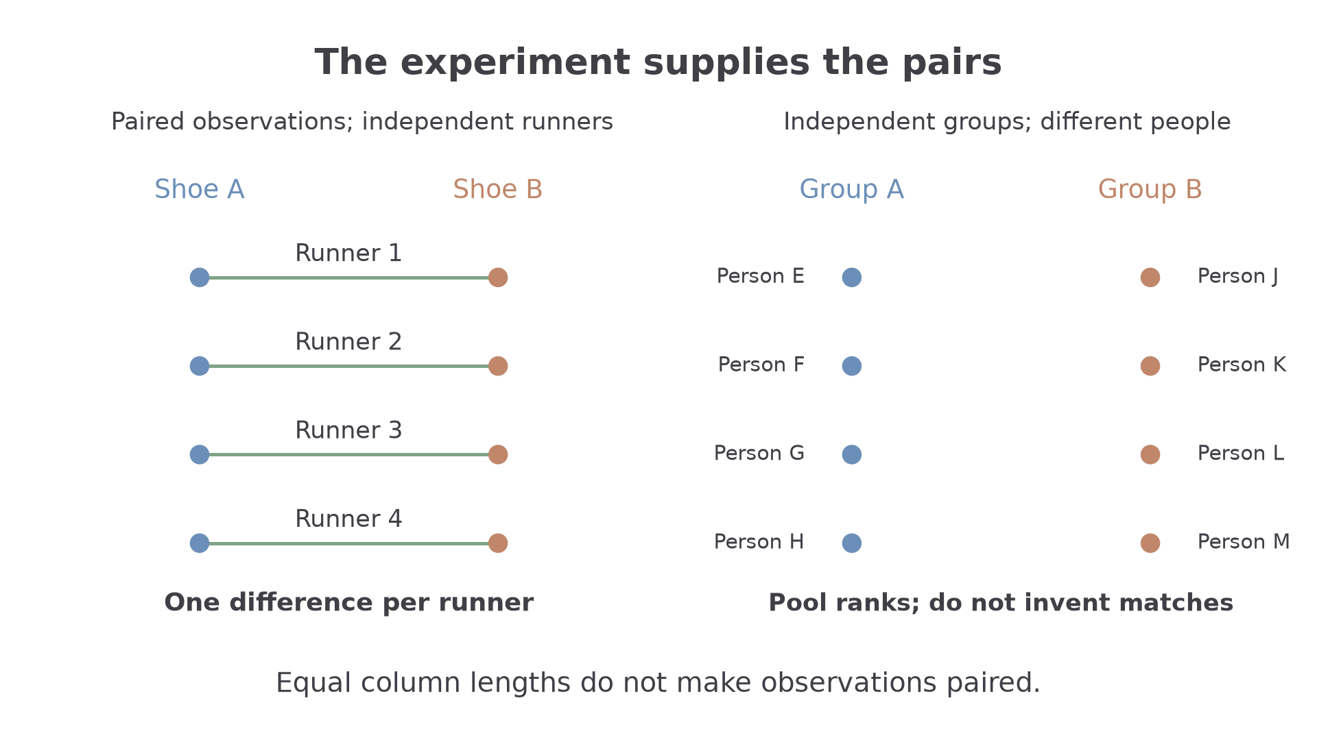
Pair only when the experiment provides a meaningful match

The connecting lines are part of the experiment, not something to add after sorting the values.

Paired and independent samples

Paired samples contain observations with a meaningful one-to-one match, such as before and after measurements on the same person or outcomes for deliberately matched units. Analyse their within-pair differences. Independent samples come from separate groups with no such match; analyse the two samples without inventing pairs.

Equal sample sizes do not make data paired. Conversely, paired observations can be dependent within each pair while the pair differences remain independent across randomly selected units. Before stating hypotheses, define the difference direction, for example $D=\text{after}-\text{before}$ . A reduction then means a negative median difference.

For paired sign and signed-rank tests, the parameter is the population median of the differences. This is not automatically the difference of two population medians. For independent rank-sum tests, the basic null hypothesis is that the two population distributions are identical. Interpreting a rank-sum result as a comparison of medians requires the populations to have the same shape and spread, apart from a possible location shift.

Key idea

Choose the test from how the data were collected: genuine matches lead to differences; independent groups lead to pooled ranks.

The tempting shortcut below creates pairs by numerical order. Locate the first step that changes the experimental design.

The paired sign test

Once genuine pair differences have been calculated, a paired sign test is a one-sample sign test on those differences. The sample size is the number of pairs, not the number of individual measurements.

Suppose a random sample of people completes a task before and after training. Define $D=\text{before time}-\text{after time}$ , so a positive difference means an improvement. The null hypothesis of no median improvement is $\mathrm{H}_0:m_D=0$ , where $m_D$ is the population median difference. It does not assert that every person has no change.

Paired sign-test model

For $n$ independent non-zero pair differences from a continuous population, under $\mathrm{H}_0:m_D=0$ ,

S=\text{number of positive differences} \sim\mathrm{B}(n,1/2)

Choose the binomial tail to match the defined difference direction and the alternative. No symmetry assumption is needed.

The binomial formula is supplied, but this model and its interpretation must be established from the design.

Not in the formula booklet: learn it.

In each example, the displayed differences belong to separate independently selected people. None is zero.

Worked example 1: improvement after training

Question. For $12$ randomly selected people, the before-minus-after task times, in seconds, are

2,5,-3,1,7,4,9,-6,8,10,11,12

Test at the $5\%$ significance level whether the population median time reduction is positive.

Plan. Count positive differences and use an upper binomial tail for the median reduction.

\begin{aligned} \mathrm{H}_0&:m_D=0,\quad\mathrm{H}_1:m_D>0 &&m_D\text{ is median time reduction}\\ S&\sim\mathrm{B}(12,1/2),\quad s=10 &&\text{twelve independent pairs}\\ p&=\mathrm{P}(S\ge10)=\frac{66+12+1}{4096} &&\text{include all more extreme counts}\\ &=0.019287\ldots<0.05 &&\text{one-sided comparison} \end{aligned}

Why this step? A positive before-minus-after difference is a reduction, so improvement corresponds to many positive signs. Reversing the subtraction would reverse the tail.

Answer. Reject $\mathrm{H}_0$ . There is significant evidence of a positive population median reduction in task time after training.

Check. There are $10$ positive and $2$ negative differences, totalling $12$ pairs, not $24$ independent observations.

Worked example 2 changes just one result, from a reduction of $12$ seconds to an increase of $12$ seconds. The sign count changes while the other pair differences stay fixed.

Worked example 2: one different pair changes the decision

Question. In the preceding experiment, replace the final difference $12$ by $-12$ . Repeat the same $5\%$ test.

Plan. Retain the hypotheses and sample size, but use the revised count of positive differences.

\begin{aligned} \mathrm{H}_0&:m_D=0,\quad\mathrm{H}_1:m_D>0 &&\text{same population question}\\ s&=9 &&\text{one fewer positive difference}\\ p&=\mathrm{P}(S\ge9)=\frac{220+66+12+1}{4096} &&S\sim\mathrm{B}(12,1/2)\\ &=0.072998\ldots>0.05 &&\text{outside rejection region} \end{aligned}

Why this step? The magnitude $12$ does not enter a sign test. Only its changed direction matters.

Answer. Do not reject $\mathrm{H}_0$ . There is insufficient evidence of a positive population median time reduction after training.

Check. Weakening the evidence for improvement has increased the upper-tail probability, as it should.

A two-sided paired sign test works in the same way as its single-sample counterpart: include both equally extreme tails, or compare the relevant one-tail probability with half the stated significance level.

Watch out

Wrong: “The median before minus the median after must equal the median of the pair differences.” Medians do not obey that subtraction rule in general. State hypotheses about $m_D$ , the population median of the defined within-pair difference.

This check changes the sample size and improvement count. Keep the pair interpretation when using the supplied critical region.

The matched-pairs signed-rank test

If the population of pair differences is continuous and symmetric, retain more information by ranking their magnitudes. It is the distribution of the differences that needs symmetry, rather than each of the two original measurement populations separately.

For example, different runners can have very different baseline speeds while their shoe-to-shoe time differences form a much tighter, approximately symmetric population. Define $D=\text{time in shoe A}-\text{time in shoe B}$ ; positive $D$ means shoe B is faster. Each runner supplies one difference, and runners are sampled independently.

Matched-pairs signed-rank procedure

Under $\mathrm{H}_0:m_D=0$ , rank the non-zero absolute pair differences, then calculate

W^+=\sum\text{positive ranks},\qquad W^-=\sum\text{negative ranks},\qquad T=\min(W^+,W^-)

For independent differences from a continuous symmetric population, with no tied absolute differences, use the signed-rank critical-value table. Reject for $T\le c$ , with the appropriate direction for a one-sided alternative.

The definitions of the rank sums, the statistic and the critical-value table are supplied.

In the formula booklet.

The calculations below use the booklet's two-tail $5\%$ critical value $3$ for $n=8$ .

Worked example 3: comparing two shoes on the same runners

Question. For $8$ randomly and independently selected runners, the shoe-A-minus-shoe-B time differences are

-7,-3,1,2,4,5,6,8

Assume the population of differences is continuous and symmetric. Test, at the $5\%$ significance level, whether its median differs from zero.

Plan. Test the median difference using signed ranks of the eight within-runner differences.

\begin{aligned} \mathrm{H}_0&:m_D=0,\quad\mathrm{H}_1:m_D\ne0 &&m_D\text{ is median time difference}\\ r&=(7,3,1,2,4,5,6,8) &&\text{rank absolute differences}\\ W^-&=7+3=10 &&\text{negative ranks}\\ W^+&=36-10=26 &&\text{remaining ranks}\\ T&=10>3 &&\text{two-tail }5\%\text{ comparison} \end{aligned}

Why this step? The first difference has magnitude $7$ , so it receives rank $7$ , even though it is the smallest signed value.

Answer. Do not reject $\mathrm{H}_0$ . There is insufficient evidence of a non-zero population median shoe-A-minus-shoe-B time difference.

Check. The ranks total $36$ , and both sign sums have been considered.

Worked example 4 changes only the sign of the first runner's difference. The largest negative rank now becomes positive.

Worked example 4: a small negative rank sum

Question. Replace the first difference $-7$ by $7$ , keeping the other differences and assumptions unchanged. Repeat the two-sided $5\%$ test.

Plan. Move rank $7$ to the positive group and compare the new smaller sum with the same critical value.

\begin{aligned} \mathrm{H}_0&:m_D=0,\quad\mathrm{H}_1:m_D\ne0 &&\text{same median-difference hypotheses}\\ W^-&=3 &&\text{only the }-3\text{ difference is negative}\\ W^+&=36-3=33 &&\text{positive rank sum}\\ T&=3\le3 &&\text{critical value included} \end{aligned}

Why this step? Seven positive signs are now supported by nearly all the large ranks. The single negative difference carries only rank $3$ .

Answer. Reject $\mathrm{H}_0$ . There is significant evidence of a non-zero population median difference between the times in the two shoes.

Check. The one negative rank is $3$ , so $T=3$ , not the count $1$ . Counts belong to a sign test.

Continue this lesson.

You’re previewing NovaLearn without an account. Create a free account to read the rest.

Create free account

Last Accessed

Pure Core

Statistics

Mechanics

Discrete Mathematics

Additional Pure Mathematics

5.07d, 5.07e - Paired-sample and two-sample tests

Paired or independent samples

The paired sign test

The matched-pairs signed-rank test

Continue this lesson.

Learn faster with Nova