Paper 5 - Linearising power laws and exponentials | Cambridge A-Level Physics

Learn to choose derived quantities that turn physical relationships into straight lines. Use ordinary and logarithmic axes to determine constants, keeping units, logarithm bases and intercept meanings consistent.

Choosing quantities that make a straight line

Can a curved graph obey a simple law perfectly? Yes: the curve may be the right relationship plotted using the wrong quantities for a straight-line test. The task is to choose the axes from the equation, rather than demand a straight line from every pair of raw readings.

Start with the supplied physical model and rearrange it into $Y=GX+c$ . Identify the complete expression that will be plotted vertically as $Y$ and horizontally as $X$ . Then equate the coefficient of $X$ to the gradient $G$ and the remaining constant to the intercept $c$ . Axis choices determine both the algebra and the units. Paper 5 supplies the necessary model in the task; do not assume that Paper 4's formula pages accompany it.

For example, an oscillating spring system is modelled by

T^2=\frac{4\pi^2}{k}(m+m_{\mathrm e}) =\frac{4\pi^2}{k}m+\frac{4\pi^2m_{\mathrm e}}{k}

Here $T$ is period in seconds, $m$ the added mass in kilograms, $k$ spring constant in $\mathrm{N\,m^{-1}}$ and $m_{\mathrm e}$ a constant effective additional mass in kilograms. The model is provided for this example, including the effective mass; it is not a new formula to memorise.

Plot $T^2$ , in $\mathrm{s^2}$ , vertically against $m$ , in kilograms. Then

G=\frac{4\pi^2}{k},\qquad c=Gm_{\mathrm e},\qquad k=\frac{4\pi^2}{G},\qquad m_{\mathrm e}=\frac{c}{G}

A straight line supports the proposed form; it need not go through the origin. The gradient unit is $\mathrm{s^2\,kg^{-1}}$ . Its reciprocal has unit $\mathrm{kg\,s^{-2}}=\mathrm{N\,m^{-1}}$ , as required for $k$ .

For $G=0.790\,\mathrm{s^2\,kg^{-1}}$ and $c=0.0395\,\mathrm{s^2}$ , the constants are $k=50.0\,\mathrm{N\,m^{-1}}$ and $m_{\mathrm e}=0.0500\,\mathrm{kg}$ . The squared-period intercept is not itself a mass: its units immediately expose that tempting mistake.

Other supplied forms suggest other transformations. If $y=a/x+b$ , plot $y$ against $1/x$ . If $y^2=ax+b$ , plot $y^2$ against $x$ . If $y=a(x+b)^2$ , with $a>0$ and $x+b>0$ throughout the range, plot $\sqrt y$ against $x$ ; the gradient is $\sqrt a$ , not $a$ . Choose the transformation before completing the derived-data columns.

Exam tip

Write the actual axis quantities beside the rearranged equation. “Compare with $y=mx+c$ ” earns no graph-analysis credit if it never identifies which measured or derived quantity belongs on each axis.

Finding an exponent with logarithms

A power law can become a straight line even when its exponent is unknown. A logarithm turns multiplication into addition and brings an exponent down as a multiplier. Use positive numerical ratios so that every logarithm has a dimensionless argument.

For a positive number $u$ , $\lg u$ is its base-ten logarithm: $10^{\lg u}=u$ . Its inverse is the calculator's power-of-ten operation, not multiplication by ten. The natural logarithm $\ln u$ has base $e$ . For positive $u,v$ , either consistent logarithm base obeys

\log(uv)=\log u+\log v,\quad \log(u/v)=\log u-\log v,\quad \log(u^n)=n\log u

These identities are mathematical tools to recall; they are not supplied physics formulae. Zero and negative arguments have no real logarithm, so a logarithmic plot cannot silently include such readings.

Suppose a positive period and mass obey the supplied empirical form

\frac{T}{\mathrm s}=A\left(\frac{m}{\mathrm{kg}}\right)^n

Here $A$ and $n$ are dimensionless numerical constants for the stated units. Taking base-ten logarithms gives

\lg(T/\mathrm s)=n\lg(m/\mathrm{kg})+\lg A

Thus a graph of $\lg(T/\mathrm s)$ against $\lg(m/\mathrm{kg})$ has gradient $n$ and intercept $c=\lg A$ , so $A=10^c$ . The axes and gradient are dimensionless. Equivalently, in $T=Km^n$ , the dimensional coefficient is $K=A\,\mathrm s\,\mathrm{kg}^{-n}$ . Its units depend on the exponent.

[DIAGRAM: asset_name: A power law on ordinary and logarithmic axes; asset_slug: practical-a2-power-law; caption: The curved period-mass relationship becomes a straight log-log line whose gradient is the exponent; description: Two panels show the model T in seconds equals 0.500 times the square root of m in kilograms. Ordinary axes show a square-root curve. Logarithmic-quantity axes show lg of T over seconds against lg of m over kilograms as a line of gradient 0.500 and intercept minus 0.3010. The unit ratios inside the logarithms are explicit.]
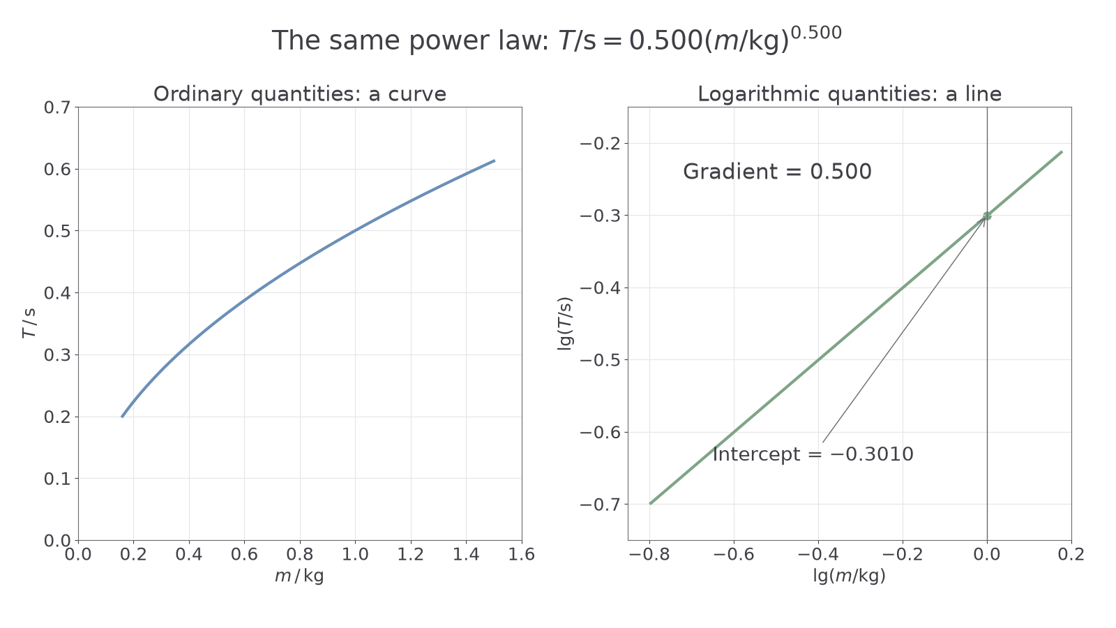
The curved period-mass relationship becomes a straight log-log line whose gradient is the exponent

For that line, $n=0.500$ and $A=10^{-0.3010}=0.500$ . A mass of $0.400\,\mathrm{kg}$ gives $T=0.500\sqrt{0.400}=0.316\,\mathrm s$ . If mass were expressed in grams instead, $\lg(m/\mathrm{kg})=\lg(m/\mathrm g)-3$ : the gradient stays $0.500$ , but the intercept becomes $-1.8010$ . An intercept is meaningful only with its stated axes and units.

Continue this lesson.

You’re previewing NovaLearn without an account. Create a free account to read the rest.

Create free account

Last Accessed

AS foundations

AS practical skills

AS mechanics

AS waves

AS electricity

AS particles

A Level mechanics

A Level thermal physics

A Level oscillations

A Level fields and circuits

A Level quantum and nuclear physics

A Level applications

A Level practical skills

Paper 5 - Linearising power laws and exponentials

Choosing quantities that make a straight line

Finding an exponent with logarithms

Continue this lesson.

Learn faster with Nova