1.3 - Combining uncertainties | Cambridge A-Level Physics

Express measurement uncertainty in absolute, fractional and percentage forms. Combine uncertainties in calculated quantities, including differences, products, quotients and powers, and explain why a small difference can be much less certain than either original reading.

Absolute and percentage uncertainty

Can two carefully measured lengths give a rather uncertain extension? Yes: subtracting two large, nearly equal readings can leave a small difference with a surprisingly large percentage uncertainty. We need to track the uncertainty as well as the value.

A measurement reported as $(50.0\pm0.5)\,\mathrm{mm}$ has value $50.0\,\mathrm{mm}$ and absolute uncertainty $0.5\,\mathrm{mm}$ . The uncertainty has the same unit as the measured quantity. The stated interval runs from $49.5\,\mathrm{mm}$ to $50.5\,\mathrm{mm}$ . It expresses an estimate of measurement uncertainty, not a guarantee about the true value.

To compare measurements of different sizes, divide the uncertainty by the magnitude of the value. Multiplying this fraction by 100 expresses it as a percentage.

Fractional and percentage uncertainty

\text{fractional uncertainty}=\frac{\Delta x}{|x|} \qquad \text{percentage uncertainty}=\frac{\Delta x}{|x|}\times100\%

Here $x$ is the reported quantity and $\Delta x$ its absolute uncertainty, in the same unit. The fraction is dimensionless. The uncertainty is non-negative. This use of $\Delta x$ means an uncertainty; in other contexts $\Delta x$ can mean a change, so read the definition.

Not on the data sheet: learn it.

For $(50.0\pm0.5)\,\mathrm{mm}$ , the fractional uncertainty is $0.5/50.0=0.010$ , or $1.0\%$ . Converting both lengths to metres leaves the fraction unchanged: $0.0005/0.0500=0.010$ . A percentage uncertainty is not measured in millimetres or metres.

Worked example 1: converting a percentage back to an interval

Question. A current of $0.240\,\mathrm{A}$ has a percentage uncertainty of $3.0\%$ . Find the absolute uncertainty.

Plan. Turn the percentage into a fraction before multiplying by the measured value.

\Delta I=\frac{3.0}{100}\times0.240\,\mathrm{A} =0.0072\,\mathrm{A}

Answer. $0.0072\,\mathrm{A}$ , or approximately $0.007\,\mathrm{A}$ at one significant figure. A corresponding rounded report is $(0.240\pm0.007)\,\mathrm{A}$ .

Check. The uncertainty is much smaller than the reading, as a few per cent should be.

Percentage change uses the same division idea but answers a different question: an increase from $20\,\mathrm{cm}$ to $23\,\mathrm{cm}$ is $(23-20)/20\times100\%=15\%$ . That is a change relative to an initial value, not automatically an uncertainty.

Useful symbols help you state comparisons precisely. $\Delta x\ll |x|$ means the uncertainty is much smaller than the magnitude of the reading; $\gg$ means much greater than, $\le$ means less than or equal to, and $\ge$ means greater than or equal to. Use $\approx$ for an approximation and $\propto$ for proportionality. A value close to zero can have a large or undefined percentage uncertainty even when its absolute uncertainty is small.

Watch out

A $4\%$ uncertainty is a fraction of 0.04, not 4. Multiplying a reading by 4 would give a 400% uncertainty. Keep the percentage sign until you deliberately divide by 100.

Check both forms of a new measurement.

Uncertainty in sums and differences

When adding or subtracting measured quantities, consider the combination that makes the calculated result as high or as low as possible. For a difference, one reading can be too high while the other is too low. The uncertainty therefore adds even though the values subtract.

Sums and differences

y=a+b\quad\text{or}\quad y=a-b \qquad\Rightarrow\qquad \Delta y=\Delta a+\Delta b

The quantities being added or subtracted must have compatible units. $\Delta a$ , $\Delta b$ and $\Delta y$ are non-negative absolute uncertainties in that same unit. This is the simple worst-case combination used here.

Not on the data sheet: learn it.

Suppose a spring's loaded length is $(100.0\pm0.5)\,\mathrm{mm}$ and its unloaded length is $(80.0\pm0.5)\,\mathrm{mm}$ . Its extension is $20.0\,\mathrm{mm}$ . The largest possible difference within these intervals is $100.5-79.5=21.0\,\mathrm{mm}$ ; the smallest is $99.5-80.5=19.0\,\mathrm{mm}$ . The extension is therefore $(20.0\pm1.0)\,\mathrm{mm}$ .

[DIAGRAM: asset_name: A difference keeps both uncertainties; asset_slug: difference-uncertainty; caption: Opposite shifts in the two readings give the extreme values of their difference; description: Two interval bars show unloaded length 80.0 plus or minus 0.5 millimetres and loaded length 100.0 plus or minus 0.5 millimetres. A second panel shows the resulting extension interval from 19.0 to 21.0 millimetres centred at 20.0. The maximum extension uses the largest loaded and smallest unloaded lengths; the minimum uses the opposite endpoints.]
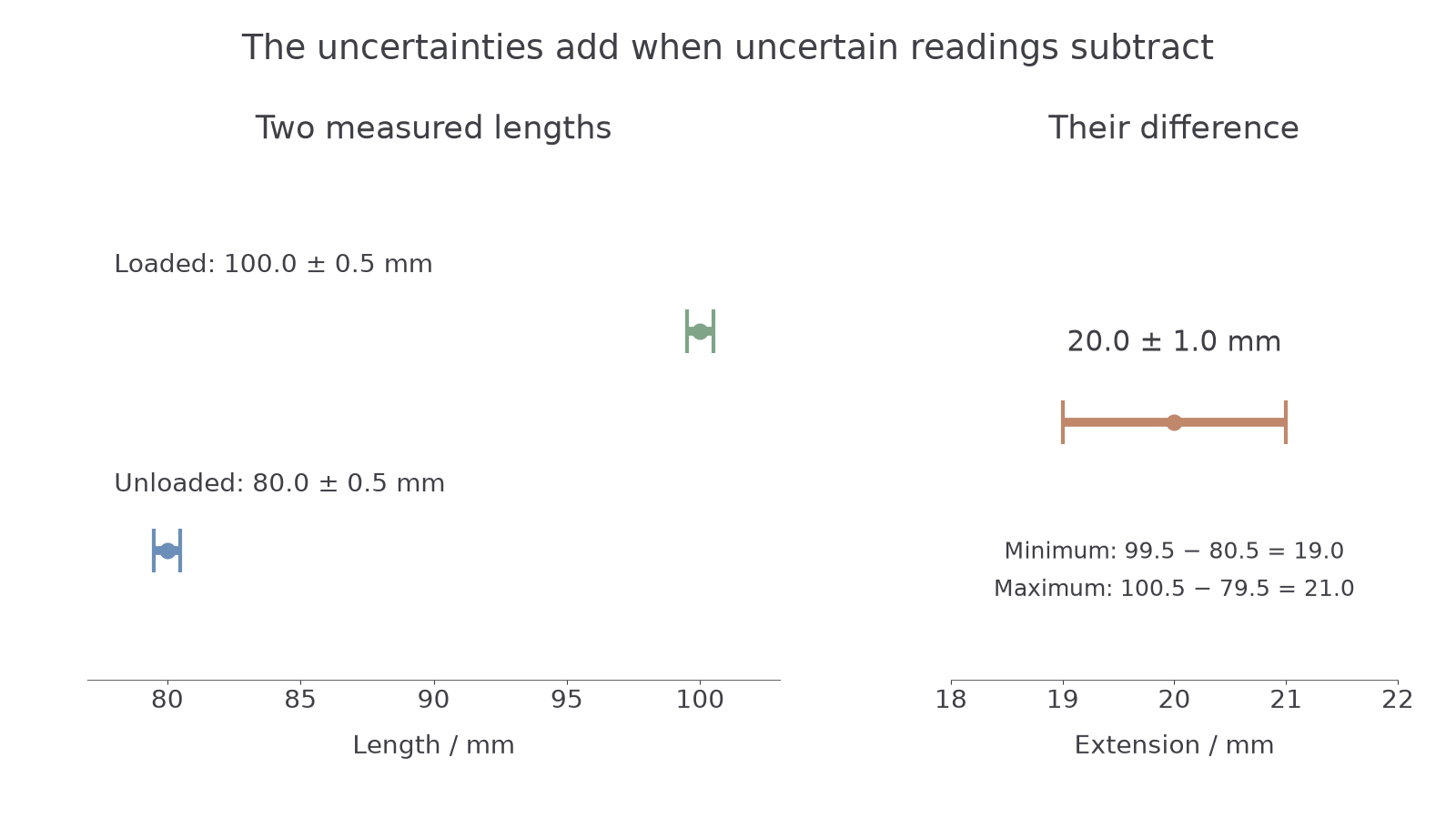
Opposite shifts in the two readings give the extreme values of their difference

The loaded reading has percentage uncertainty $0.5\%$ ; the extension has percentage uncertainty $1.0/20.0\times100\%=5.0\%$ . The small difference is ten times less certain in percentage terms. That is why a practical method should often produce a substantial extension rather than a barely visible one.

Model limit

The simple addition rules give a conservative estimate based on extreme changes. They are not a statistical confidence interval. When a question supplies an uncertainty convention or a special relationship between errors, use that information rather than assuming the errors are independent.

Shared systematic errors need particular care. If the same constant ruler-zero offset is present in two length readings, it cancels when you subtract the readings. Two separate endpoint-reading uncertainties do not cancel just because the values subtract. You must identify what each uncertainty represents.

Worked example 2: total length

Question. Two separately measured strips have lengths $(12.4\pm0.1)\,\mathrm{cm}$ and $(8.2\pm0.1)\,\mathrm{cm}$ . Calculate their total length and its absolute uncertainty.

Plan. Add the lengths and add their absolute uncertainties.

L=12.4+8.2=20.6\,\mathrm{cm} \qquad \Delta L=0.1+0.1=0.2\,\mathrm{cm}

Answer. $(20.6\pm0.2)\,\mathrm{cm}$ .

Check. The largest permitted total is $12.5+8.3=20.8\,\mathrm{cm}$ , matching the upper limit.

Now use subtraction without subtracting the uncertainties.

Uncertainty in products and powers

Multiplication and division scale a result, so relative uncertainty is the useful measure. A distance that is 1% high makes a calculated speed 1% high; a time that is 1% low also makes that speed approximately 1% high. The adverse effects add.

Products, quotients and powers

y=Kab\quad\text{or}\quad y=K\frac{a}{b} \qquad\Rightarrow\qquad \frac{\Delta y}{|y|}\approx\frac{\Delta a}{|a|}+\frac{\Delta b}{|b|}

For $y=Ka^{n}$ ,

\frac{\Delta y}{|y|}\approx |n|\frac{\Delta a}{|a|}

Here $K$ is an exact constant, $n$ a known exponent, and all fractions are dimensionless. The same addition works with percentages. These are simple approximate rules for small relative uncertainties; combine powers and products by adding their contributions.

Not on the data sheet: learn it.

The absolute size of the exponent matters. A reciprocal has power $-1$ , so its percentage uncertainty is unchanged. A square doubles a percentage uncertainty; a square root, power $1/2$ , halves it. Exact factors such as 2 and $\pi$ add no measurement uncertainty.

Worked example 3: a speed from uncertain measurements

Question. A measured distance is $(32.0\pm0.2)\,\mathrm{m}$ and a measured time is $(4.00\pm0.10)\,\mathrm{s}$ . Calculate the speed and its uncertainty using the simple percentage rule.

Plan. Calculate the value, add fractional uncertainties, then convert the result back to an absolute uncertainty.

\begin{aligned} v&=\frac{32.0\,\mathrm{m}}{4.00\,\mathrm{s}}=8.00\,\mathrm{m\,s^{-1}}\\ \frac{\Delta v}{v}&\approx\frac{0.2}{32.0}+\frac{0.10}{4.00}=0.03125\\ \Delta v&\approx0.03125\times8.00=0.25\,\mathrm{m\,s^{-1}} \end{aligned}

Answer. $(8.00\pm0.25)\,\mathrm{m\,s^{-1}}$ , retaining two significant figures in the uncertainty.

Check. The time contributes $2.5\%$ , more than the distance's $0.625\%$ . Improving the timing would help most.

Powers matter whenever a measurement controls an area or volume.

Exam-style example: uncertainty from a diameter

Question. A circular wire has diameter $(0.500\pm0.005)\,\mathrm{mm}$ . Use $A=\pi d^{2}/4$ to calculate its cross-sectional area in square metres and estimate the absolute uncertainty in the area.

Plan. Convert the diameter to metres, square it to find area, then double its fractional uncertainty.

\begin{aligned} A&=\frac{\pi(0.500\times10^{-3}\,\mathrm{m})^{2}}{4} =1.9635\times10^{-7}\,\mathrm{m^{2}}\\ \frac{\Delta A}{A}&\approx2\frac{0.005}{0.500}=0.020\\ \Delta A&\approx0.020(1.9635\times10^{-7}) =3.927\times10^{-9}\,\mathrm{m^{2}} \end{aligned}

Answer. Approximately $(1.96\pm0.04)\times10^{-7}\,\mathrm{m^{2}}$ .

Check. A 1% diameter uncertainty becomes a 2% area uncertainty. The exact factor $\pi/4$ adds none.

You also need to reverse powers when rearranging equations. From $A=\pi d^{2}/4$ , isolate the square first, then take the positive square root for a physical diameter:

d^{2}=\frac{4A}{\pi} \qquad\Rightarrow\qquad d=\sqrt{\frac{4A}{\pi}}

An nth root is the power $1/n$ ; a reciprocal is the power $-1$ . Use calculator brackets around the entire numerator and denominator before taking a root. To find an arithmetic mean, add the values and divide by their number; for example, the mean of 3.1, 3.4 and 3.4 is $9.9/3=3.3$ . A mean does not justify rounding all the original readings to one significant figure first.

Exam tip

Work with unrounded fractions until the end. Decide whether the question needs absolute uncertainty or percentage uncertainty, and include a unit only for an absolute uncertainty. Never subtract percentage uncertainties for a quotient.

Apply a squared denominator in a different experiment.

Quick Recap

Absolute uncertainty has the measurement's unit; fractional and percentage uncertainties compare it with the magnitude of the value.
Add absolute uncertainties for sums and differences.
Add fractional or percentage contributions for products and quotients; multiply each contribution by the magnitude of its power.
Convert back to an absolute uncertainty when reporting a value with a plus-or-minus interval.

Two precise length readings can give an uncertain extension because their absolute uncertainties combine while their difference is small.

Last Accessed

AS foundations

AS practical skills

AS mechanics

AS waves

AS electricity

AS particles

A Level mechanics

A Level thermal physics

A Level oscillations

A Level fields and circuits

A Level quantum and nuclear physics

A Level applications

A Level practical skills

1.3 - Combining uncertainties

Absolute and percentage uncertainty

Uncertainty in sums and differences

Uncertainty in products and powers

Quick Recap

Learn faster with Nova