9.1 - Charge, current and drift velocity

Moving charge and conventional current

How can a metal wire carry several amperes when its electrons' average drift is much slower than a walking pace? A large current does not require each carrier to travel quickly: a wire contains an enormous number of mobile carriers. First separate the motion of those carriers from the amount of charge each one carries.

An electric current is a flow of charge carriers. In a metal, mobile electrons move through a lattice of positive ions. The ions vibrate about fixed positions; they do not travel around the circuit. In an electrolyte, positive and negative ions can both carry current. A charged object sitting still has charge but does not, by that fact alone, constitute a current.

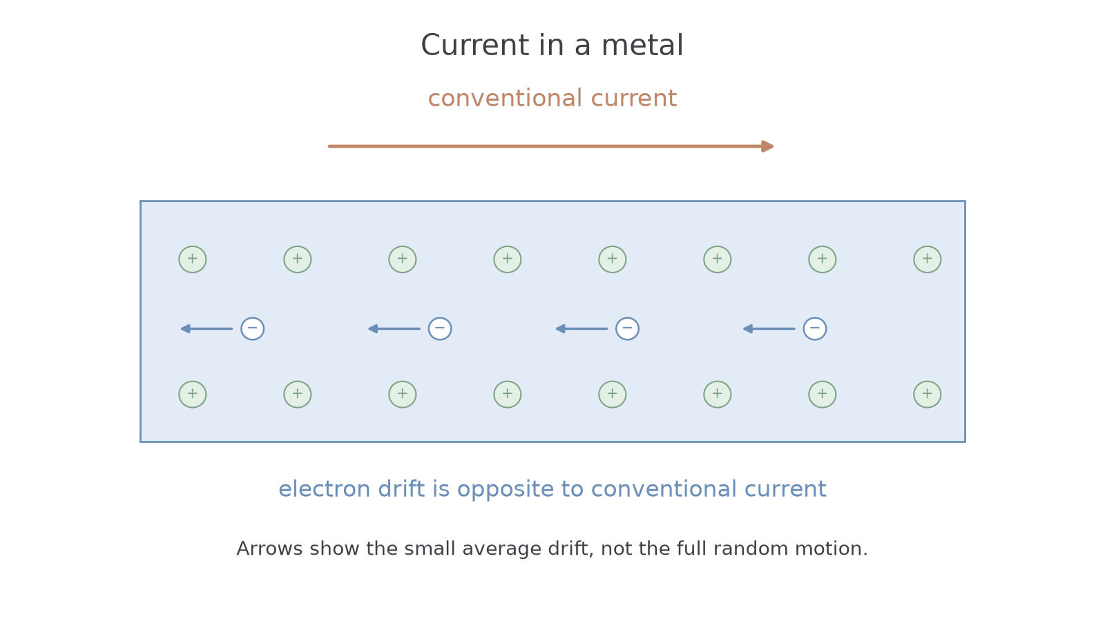
Conventional current is in the direction a positive charge would move. Metal electrons are negatively charged, so their drift direction is opposite to conventional current. In an electrolyte, a negative ion moving one way and a positive ion moving the opposite way can contribute to current in the same conventional direction.

[DIAGRAM: asset_name: Carrier motion and conventional current; asset_slug: electricity-carrier-direction; caption: In a metal, electron drift and conventional current have opposite directions; description: A straight section of metal wire contains pale positive lattice ions at fixed sites and small negative electron symbols. Blue arrows show a leftward average electron drift. A clay arrow above the wire shows conventional current to the right. A note says the arrows represent average drift, not the electrons' full random motion.]

Charge comes in discrete amounts. An electron has charge $-e$, while a proton has charge $+e$, where the elementary charge has magnitude $e=1.60\times10^{-19}\,\mathrm{C}$ using the examination value. A doubly charged ion has magnitude $2e$. The coulomb, C, is the SI unit of charge.

For a transfer of $N$ electrons, the magnitude of charge transferred is $Q=Ne$. Here $N$ is an integer count; $Q$ is in C and $e$ is in C. This counting relation is not printed on the general data sheet, although $e$ is supplied. Macroscopic values can look continuous because an elementary charge is so small.

A direction statement should name which thing is moving. “The electrons move right” and “the current is right” describe opposite physical cases in an ordinary metal.

Current as charge per unit time

To measure current, imagine a fixed cross-section through a wire and count the net charge passing it each second. You are counting a flow through a location, rather than all the charge contained in the wire.

If $6\,\mathrm{C}$ passes in $3\,\mathrm{s}$, the average current is $2\,\mathrm{A}$. A larger current means more charge passes per unit time; a longer time at the same current means a larger total transferred charge.

A varying current needs its actual history. If the current is $2.0\,\mathrm{A}$ for 3 seconds and then $0.50\,\mathrm{A}$ for 4 seconds, the total charge is $2.0\times3+0.50\times4=8.0\,\mathrm{C}$. The final current alone does not describe the whole interval.

For a current that increases uniformly from zero to $0.60\,\mathrm{A}$ over $4.0\,\mathrm{s}$, the current–time area is a triangle. Its charge is $Q=\tfrac12\times4.0\times0.60=1.2\,\mathrm{C}$. Equivalently, the average current is $(0+0.60)/2=0.30\,\mathrm{A}$, which gives the same charge. Using the final $0.60\,\mathrm{A}$ throughout would incorrectly count a full rectangle and double the transfer. If a steady interval follows, add its rectangular area to this triangular area.