Paper 3 - Trend lines, gradients and constants
Learn to choose a trend line, obtain a reliable gradient and intercept, and turn those graph features into physical constants. You will also use a tangent to describe how a changing quantity behaves at one instant.
Straight trends, curves and tangents
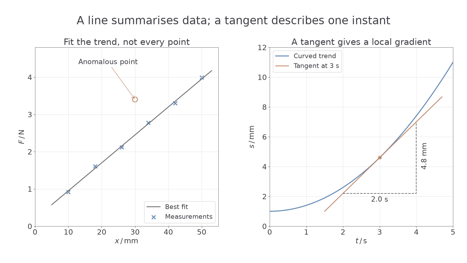
Should a good line pass through every measured point? Usually it should not. Random measurement variations scatter points around the underlying relationship, so chasing every point can turn a simple physical trend into an imaginary zigzag.
When the data support a straight relationship, draw a fine, continuous line of best fit with points distributed reasonably evenly on either side across its length. Use the whole pattern rather than joining the first and last measurements. Do not force the line through the origin unless the data and the physical model justify it. An offset may be the clue the experiment is meant to reveal.
A point far from the trend may be anomalous. Recheck its measurement and calculation, and repeat it if possible. If you exclude a clearly anomalous point when drawing the line, identify it visibly by circling or labelling it. Do not silently remove a point just because it makes the result less convenient.
A systematic bend needs a smooth curved trend line, rather than a straight line with excuses. Draw the curve through the overall pattern without kinks. To find the curve's gradient at a chosen point, draw a tangent with the same local direction there. Make it long enough to calculate its gradient using widely separated coordinates. A line joining two widely separated points on the curve gives an average gradient, which is a different quantity.
[DIAGRAM: asset_name: A best fit and a tangent; asset_slug: p3-trends-and-tangent; caption: Scatter calls for a best fit, while a curved trend needs a tangent for a local gradient; description: The left graph shows a straight force-extension trend with six scattered measurements and one labelled anomalous point. A fine best-fit line balances the ordinary points rather than joining them. The right graph shows displacement in millimetres increasing as one plus 0.4 times time squared, with a tangent at three seconds; two separated points on the tangent define its gradient triangle.]
Watch out
A tangent is a straight line matching the curve's direction at the chosen point. It is not a line drawn from the origin to that point, and it need not pass through any measured data point apart from its contact with the fitted curve.
For example, a cooling curve becomes flatter with time. A tangent early in cooling has a negative gradient of larger magnitude than one later. That mathematical change describes slower cooling; it is not an excuse to replace the curve by one straight line.
Gradients and intercepts from the line
The fitted line uses information from the whole dataset, so obtain its gradient from points on that line. They need not be measured points. Pick convenient coordinates separated by more than half the drawn line's length, and show the coordinate differences in your working. A large triangle makes reading uncertainty a smaller fraction of each difference.
Gradient of a straight line
Here and are coordinates on the same fitted straight line, or on the same tangent. The gradient unit is the vertical quantity's unit divided by the horizontal quantity's unit. Symbols describe graph variables here; need not mean mass.
Not on the data sheet: learn it.
A negative gradient is physically meaningful: the vertical quantity decreases as the horizontal quantity increases. Do not discard its sign. To find where two trends intersect, read the coordinates of their crossing; if their equations are known, equate their vertical expressions and solve for the horizontal coordinate.
Worked example 1: a gradient and a hidden intercept
Question. A graph of force against extension uses horizontal values from to . Points on its best-fit line are and . Determine its gradient in newtons per metre and its force-axis intercept.
Plan. Use coordinate differences, then substitute into . Convert millimetres before reporting an SI gradient.
Answer. Gradient ; intercept .
Check. Substitution of the other point gives too. The force at the left edge of the graph is not the intercept, because that edge is not .
For a tangent to displacement against time, the gradient unit is displacement per time. If its coordinate changes are in , the local rate is . The gradient comes from the tangent's coordinates, rather than a pair of points on the curved trend.
Exam tip
A false origin changes what the edge of the grid means, not the equation. If the vertical-axis intercept lies outside the plotted region, calculate using a line point and the gradient.
Now preserve the sign and the units in a different experiment.
Constants from a graph equation
A gradient becomes useful physics when you compare the plotted variables with a proposed relationship. First decide what is on each axis, then rewrite the physical equation to match a straight line. Do not assume the gradient is whichever constant the question happens to mention.
The general form describes vertical variable , horizontal variable , gradient and vertical intercept . A graph of force against extension may have gradient equal to a stiffness. The reversed graph, extension against force, has the reciprocal gradient. The axis order matters.
Worked example 2: a squared-period graph
Question. An experiment is described by the supplied relationship
where period is in seconds, length in metres, an acceleration in metres per second squared and a constant in square seconds. A graph of against has gradient and intercept . Determine and .
Plan. Match the physical equation term by term to , then rearrange the gradient expression.
Answer. and .
Check. The reciprocal gradient has acceleration units. The value is close to the usual near-Earth acceleration of free fall, about , rather than thousands of times larger.
This experiment illustrates a powerful fact: a graph can measure a physical constant without relying on one specially chosen reading. The fitted gradient combines the trend of the data. Scatter and possible systematic offsets still need assessing, as you will do in the next lesson.
A non-zero intercept does not automatically invalidate a gradient method. It may represent a fixed offset in the stated model. Judge it using the equation and apparatus, rather than erasing it by drawing through the origin.
Quick Recap
- Fit the overall pattern: a balanced straight line for a linear trend, or a smooth curve when the data require it.
- Identify an excluded anomalous point; do not silently change data.
- Use widely separated coordinates on the fitted line or tangent for a gradient, keeping its sign and units.
- Calculate an off-grid intercept from the line equation and match the physical equation to the actual axes.
A good line usually does not pass through every measurement: it represents the underlying trend while allowing for the scatter in real data.