Paper 3 - Testing relationships with uncertain data

Uncertainty from the measurement method

If two estimates of the same constant differ, must one be wrong? Not necessarily. A measurement represents a range of plausible values, and the difference may be smaller than the uncertainty of the method.

An absolute uncertainty is expressed in the same unit as the measured quantity. A reading $L=(142\pm2)\,\mathrm{mm}$ has an absolute uncertainty of $2\,\mathrm{mm}$. Its fractional uncertainty is $2/142$, and its percentage uncertainty is about 1.4%. These describe the size of the uncertainty, rather than a known error that you can subtract.

Estimate uncertainty from the actual measurement: the scale, alignment, uncertainty of locating an endpoint, variation between repeats and any other important effects. Half a smallest scale division can describe ideal reading uncertainty for a clear analogue scale, but it is not automatically the uncertainty of a whole experiment. Measuring a fuzzy shadow edge to the nearest millimetre may be uncertain by several millimetres.

For repeated measurements with genuine random variation, half their range is an appropriate simple estimate in many Paper 3 contexts. Use the mean as the central value, and consider whether resolution or another effect sets a larger minimum uncertainty. Identical digital readings do not prove zero uncertainty: changes smaller than the display step can be invisible. That is a useful limit to the apparent confidence of a steady screen.

In a difference of two measured positions, both readings can contribute uncertainty. If a length is obtained from $(381\pm1)\,\mathrm{mm}$ minus $(152\pm1)\,\mathrm{mm}$, the simple maximum uncertainty rule gives $(229\pm2)\,\mathrm{mm}$. It would be wrong to attach only one reading's uncertainty to the difference.

Comparing estimates of a constant

A proposed relationship often says that a combination of variables stays constant. Calculate that combination for different settings, then compare its variation with the uncertainty you are given. Simply saying that two numbers are “close” does not tell anyone how close is close enough.

For example, the hypothesis $y=kx$ predicts $k=y/x$. The variables must have the meaning and units stated in the experiment. Two settings provide two estimates of $k$, which can differ because of measurement uncertainty even when the hypothesis describes the observations well.

One useful comparison is the absolute difference between two estimates expressed as a percentage of their mean:

Here the two positive constant estimates have the same unit. This symmetric convention treats them equally. Use any denominator convention specified in the task; state the one you use if necessary. A comparison with a known reference value instead uses that reference as its denominator. Neither is the same as dividing an uncertainty by a measurement.

If the difference exceeds the stated criterion, the data do not support the relationship to that precision. Check measurements, controls and the model before declaring a law of physics wrong. If the difference is smaller, say “supports” or “consistent within uncertainty”, rather than “proves”. With only two settings, many other curves could also pass through the data.

Apply a new criterion to a result that goes the other way.

What the evidence can support

A useful conclusion answers the experimental question with the measured trend or constant, its unit and the relevant uncertainty. It distinguishes what you found from how strongly the evidence supports it.

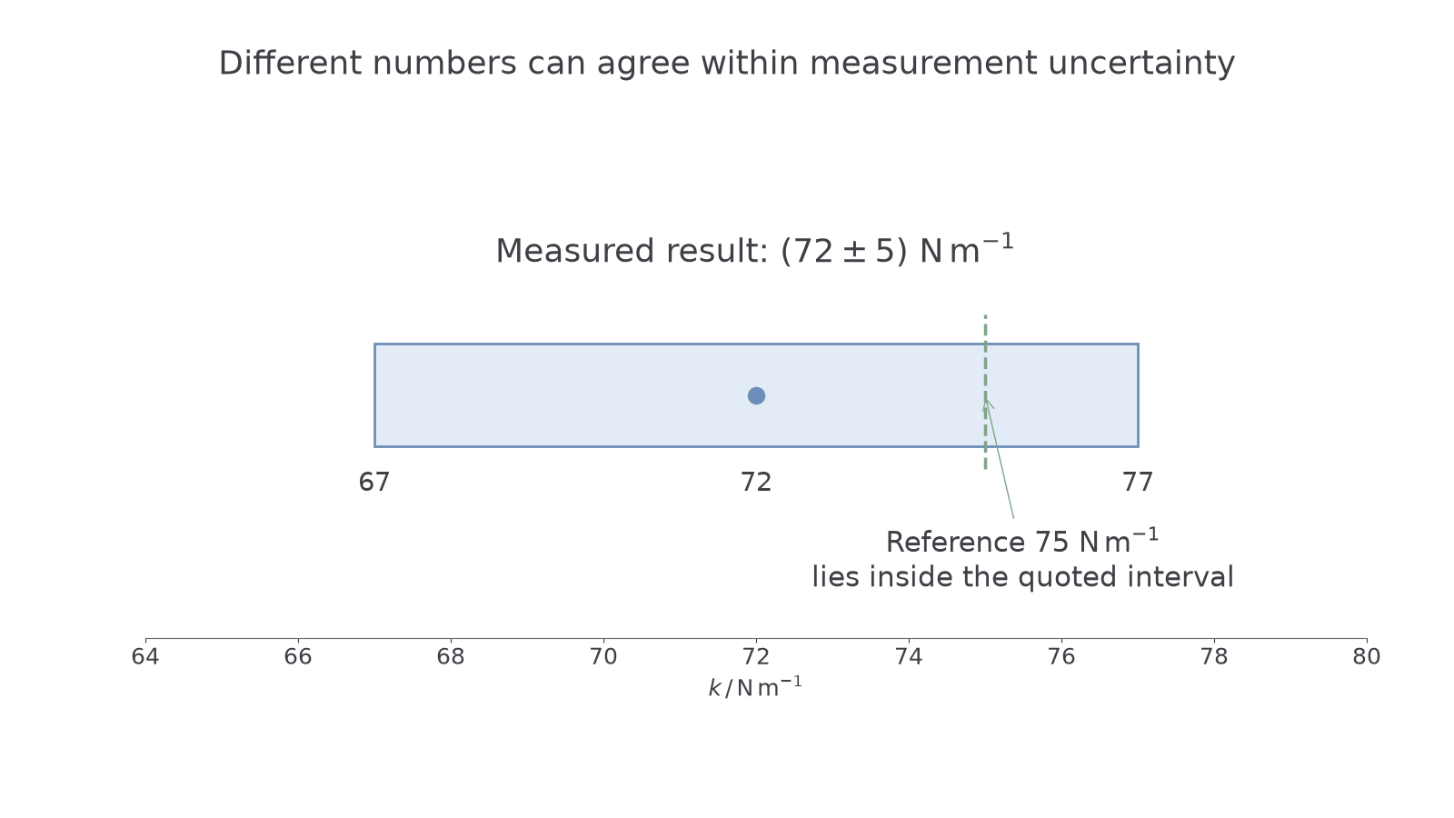
Suppose an extension $x$ and force $F$ are related by the supplied model $F=kx$. An experimental value $k=(48\pm3)\,\mathrm{N\,m^{-1}}$ reports both a central estimate and its limited precision. The value $50\,\mathrm{N\,m^{-1}}$ lies inside that quoted interval, so the result is consistent with it. This agreement does not establish that every load, temperature or material follows the same relationship.

[DIAGRAM: asset_name: A reference within an uncertainty interval; asset_slug: p3-uncertainty-interval; caption: A reference can differ from the central estimate while remaining consistent with its quoted interval; description: A horizontal shaded interval extends from 67 to 77 newtons per metre, centred on a measured value of 72 newtons per metre. A dashed reference marker at 75 newtons per metre lies inside the interval. The axis is labelled k in newtons per metre and the measured result is written as 72 plus or minus 5 newtons per metre.]

Use the result to predict another value only within conditions where the model is justified. Interpolation predicts between measured settings. Extrapolation predicts outside them and is less secure, because the relationship may change. A stretched material, for example, may stop obeying a proportional relationship at a larger load. You will study that physical limit in the materials lessons.

The opening puzzle has become a principle of experimental reasoning: different numerical estimates can still agree when their uncertainties are taken seriously. Conversely, a reassuring-looking average does not excuse a trend in the individual values.

Quick Recap

• Estimate uncertainty from the measurement method and repeats; a steady digital display does not give zero uncertainty.
• Convert between absolute and percentage uncertainty using the measured value in consistent units.
• Compare constant estimates numerically with the supplied uncertainty criterion, then state a consistent conclusion.
• Report a constant with its unit and uncertainty, and distinguish interpolation from extrapolation.

Two different estimates can both be reasonable when their difference is compatible with the experiment's uncertainty; the data support a relationship rather than proving it.