Paper 3 - Tables, precision and graph scales
Learn to turn raw readings into a clear results table, calculate with justified precision and choose graph scales that reveal a trend. Good presentation preserves what was measured so you and someone else can check the physics.
Tables that preserve the measurements
Can an extra zero change what a measurement claims? A length written as and one written as have equal numerical values, but they normally communicate different recording precision. A useful results table must preserve this information as well as the numbers.
Prepare one table before taking readings. Put the independent variable, which you deliberately change, in the first column. Include columns for every raw quantity measured, repeats where appropriate, and the quantities calculated from them. Record readings directly rather than keeping scraps and copying up a tidy selection later. Unexpected values are evidence to investigate, not inconvenient numbers to hide.
Every column needs a quantity and its unit. Writing means the numerical value of length expressed in centimetres. A cell containing 12.4 then communicates . The heading is a ratio; it is not the product of quantity and unit.
| Suitable heading | Why it works |
|---|---|
| Identifies length and its unit. | |
| Current / mA | Words can identify the quantity. |
| A squared time has a squared time unit. | |
| A dimensionless count needs no physical unit. |
“cm” alone does not identify what length was measured. “” suggests multiplication rather than the accepted heading convention. Cambridge also accepts headings such as “ (cm)” or “ in cm”, but quantity/unit is a compact, consistent choice.
Practical: timing several oscillations
A student changes a pendulum's length , times complete oscillations twice and calculates the mean period. The count is recorded once because it stays fixed.
| 20.0 | 9.0 | 9.2 | 9.10 | 0.910 |
| 30.0 | 11.0 | 10.9 | 10.95 | 1.095 |
| 40.0 | 12.7 | 12.6 | 12.65 | 1.265 |
The two measured times remain visible. A later reader can check the mean, spot the repeat spread and recompute . The extra digits in calculated columns come from calculation; they do not pretend the stopwatch displayed them.
Keep the raw readings even if a derived column will be plotted. Without them, an error in a calculation can be difficult to diagnose.
Precision in raw and calculated values
The instrument limits what a raw reading can claim. If a rule is read to the nearest millimetre, lengths in centimetres should consistently have one decimal place: , , . Writing 10 instead of 10.0 loses the stated millimetre precision; adding another zero invents finer precision.
Raw readings of the same quantity in one column use consistent decimal places suited to the instrument and method. Different instruments can require different decimal places. Calculated values follow the input precision and the operation rather than blindly matching all the decimal places in the table.
For multiplication or division in Cambridge practical work, a calculated result normally uses the same number of significant figures as the least precise measured input, or one more. If that input has significant figures, or are normally suitable. Addition and subtraction need attention to absolute precision: subtracting two lengths recorded to a millimetre does not create hundredths of a millimetre.
Worked example 1: a calculated speed
Question. A distance of is travelled in . Calculate the mean speed in metres per second and justify the precision used.
Plan. Convert to metres and use distance divided by time. Retain calculator digits until the final answer.
Answer. or . The time has two significant figures, so two or three are suitable here.
Check. About 0.4 metres in about 0.8 seconds suggests about half a metre per second. Writing 0.461728 as the final measured result would overstate the information.
Means have several common notations. For readings , the bar and angle brackets can both denote an arithmetic mean:
The summation sign means add the indicated readings; is their exact count. A square root, , reverses squaring for a non-negative quantity; a root of order , written , reverses the corresponding power, choosing the appropriate physical value. Keep these calculations unrounded until the reported result. You will use roots and means together in the gas-model lessons.
For example, repeat times of , and give . If a derived column contains , recover the period as . Similarly, a measured cube volume of corresponds to a side length . The root acts on the unit as well as the numerical value.
Watch out
Repeating the same rounded intermediate value in every later calculation can lose useful information. Show a sensible number of digits in the table, but retain guard digits while calculating from the original measurements.
Now choose the precision rather than copying a calculator display.
Graph scales and accurate points
A graph makes changes visible, so give the data enough space to show them. Usually plot the independent variable horizontally and the dependent variable vertically, unless the question specifies transformed variables or a different arrangement.
Label each axis with quantity and unit just as you label a table. Select scales that the plotted data occupy at least half of the available grid in both horizontal and vertical directions. A false origin is useful when values are far from zero: an axis for temperatures from 42 to 58 degrees Celsius need not begin at zero. Mark the actual numerical scale clearly so the apparent shape cannot be mistaken for a zero-origin plot.
Use easily read linear scales, such as 1, 2 or 5 units per large 2 cm square, with numerical labels at regular intervals no more than 2 cm apart. Avoid awkward steps such as 3 units per large square. Count the small subdivisions before plotting: they determine what a coordinate between two labels means.
[DIAGRAM: asset_name: Scales that use the graph; asset_slug: p3-useful-graph-scale; caption: A clearly labelled false origin spreads the measured temperatures across the grid; description: Two equal plotting panels show the same temperature versus time data. The left vertical scale starts at zero and compresses data between 42 and 58 degrees Celsius. The right vertical scale runs from 40 to 60 degrees Celsius and spreads the data over most of the height. Both horizontal axes run from zero to 60 seconds, axes have quantity and unit labels, and all six points are shown.]
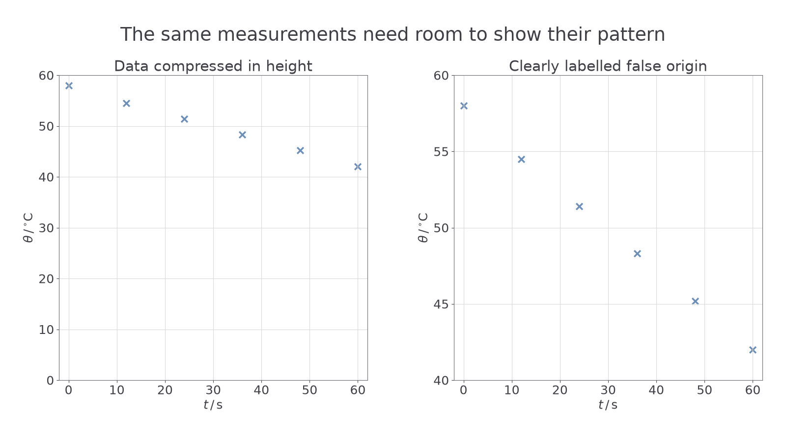
Plot every supplied or measured point carefully, to better than 1 mm on a paper grid. Use fine crosses or small encircled dots whose positions remain clear; a thick blob hides the coordinate it supposedly records. Check each point against its table row before drawing a trend line. A graph here is a record of data, not a drawing that must be made to resemble a textbook prediction.
Worked example 2: selecting a scale
Question. Six measurements span to . A graph grid is 20 cm wide. Is a scale of per 2 cm suitable horizontally? Suggest a better simple scale.
Plan. Calculate the width occupied by the 40-second data range.
At per 2 cm, the points span only 8 cm, less than half the grid. A scale of per 2 cm gives a 16 cm span, so it is suitable if the chosen axis limits include all six points.
Check. The better scale is still easy to read and leaves room for the full range, rather than merely making the graph large.
The extra zero from the opening is now useful: it preserves the precision that should survive into your table and graph.
Quick Recap
- Prepare one results table with every raw reading, repeat and useful derived quantity.
- Label columns and axes with a quantity and unit; a squared quantity needs the squared unit.
- Match raw decimal places to the instrument; calculate with guard digits and report justified significant figures.
- Choose easy scales that fill at least half the grid in each direction and plot fine, accurate points.
An extra zero can change a measurement's claimed precision: write it when the instrument supports it, and leave it out when it does not.