Paper 5 - Constants, uncertainty and conclusions

Recovering physical constants from fitted numbers

Two graphs of the same experiment can have different numerical gradients. Can they still give the same physical constant? Yes: the axes may use different scale factors. A fitted number becomes physics only after the equation, units and axis scales are restored.

Begin with the supplied model and your stated axes. Derive expressions for the gradient and intercept, then rearrange with the required physical constant as the subject. Use the fitted line rather than substituting one arbitrary pair of raw readings: the line uses the whole trend and supplies its own uncertainty estimate.

For the supplied spring-system model

a plot of $T^2$ against $m$ gives $G=4\pi^2/k$ and $c=Gm_{\mathrm e}$. Therefore $k=4\pi^2/G$ and $m_{\mathrm e}=c/G$. Here period is in seconds, mass in kilograms, $G$ in $\mathrm{s^2\,kg^{-1}}$, $c$ in $\mathrm{s^2}$, $k$ in $\mathrm{N\,m^{-1}}$ and $m_{\mathrm e}$ in kilograms. The model is supplied for the investigation, not a new recall requirement.

[DIAGRAM: asset_name: Numerical gradients depend on the axis scale; asset_slug: practical-a2-scaled-gradient; caption: The two numerical gradients describe the same physical slope after the axis factors are restored; description: Two plots show the identical line T squared equals 0.800 times m plus 0.0400 in SI units. One plots T squared over seconds squared against m over kilograms and labels numerical gradient 0.800. The other plots the same vertical quantity against m divided by 0.10 kilogram and labels numerical gradient 0.0800. Both derive physical gradient 0.800 seconds squared per kilogram.]

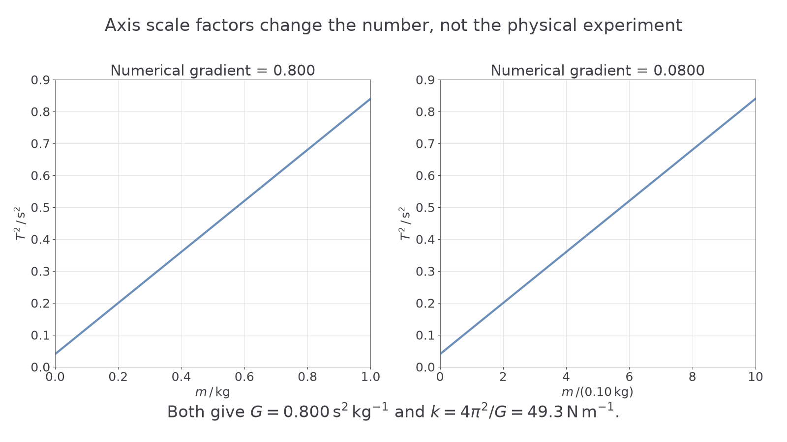
On an axis headed $m/(0.10\,\mathrm{kg})$, an increase of one plotted unit is $0.10\,\mathrm{kg}$, not $1\,\mathrm{kg}$. A numerical gradient of $0.0800$ against this axis corresponds to

The constant is then $k=4\pi^2/0.800=49.3\,\mathrm{N\,m^{-1}}$. With $c=0.0400\,\mathrm{s^2}$, $m_{\mathrm e}=0.0500\,\mathrm{kg}$. If the horizontal axis were mass in grams, its physical slope would instead be $0.000800\,\mathrm{s^2\,g^{-1}}$: converting the mass unit restores the same result.

Units are a useful independent check. Since $\mathrm{N\,m^{-1}}=\mathrm{kg\,s^{-2}}$, the reciprocal of $G$'s unit has the correct spring-constant unit. An intercept with unit $\mathrm{s^2}$ cannot be substituted as a mass. For a dimensionless log axis, the intercept itself is dimensionless; inverse logarithms and the stated reference units recover the physical amplitude.

Uncertainty follows the equation for the constant

The uncertainty in a physical constant is not necessarily just the percentage uncertainty in the gradient. Read its derived equation: every uncertain input that affects the result must be accounted for, using absolute or fractional uncertainties in the appropriate place.

Use the conservative small-uncertainty rules recalled from earlier lessons. For sums and differences, add the absolute uncertainties. For products and quotients, add fractional uncertainties. A power multiplies the fractional uncertainty by the magnitude of its exponent. These are estimated bounds, not a claim that all errors have a known statistical distribution; do not replace them by a different statistical rule unless instructed.

For example, subtracting densities $(8050\pm60)\,\mathrm{kg\,m^{-3}}$ and $(1250\pm40)\,\mathrm{kg\,m^{-3}}$ gives $(6800\pm100)\,\mathrm{kg\,m^{-3}}$. Add the absolute uncertainties before converting the difference's uncertainty into a fraction, $100/6800$. Subtracting the uncertainties would incorrectly suggest that subtracting two uncertain measurements makes their difference exact.

For the spring example, take $G=(0.800\pm0.040)\,\mathrm{s^2\,kg^{-1}}$ and $c=(0.0400\pm0.0060)\,\mathrm{s^2}$. Since $k=4\pi^2/G$, its fractional uncertainty is $0.040/0.800=0.050$, or $5.0\%$. Thus $k=(49.3\pm2.5)\,\mathrm{N\,m^{-1}}$, to consistent precision. The exact factor $4\pi^2$ and exact unit conversions add no measurement uncertainty.

For $m_{\mathrm e}=c/G$, the stated conservative estimate is

so $m_{\mathrm e}=(0.050\pm0.010)\,\mathrm{kg}$. The slope and intercept have separate graphical uncertainty estimates. Do not assume their percentages are equal. Where a task specifies an extreme-value method, use the compatible limiting fitted values and show the substitutions; gradient and intercept from one fitted line are linked, so do not describe every arbitrary combination as a possible actual line.