18.5 - Electric potential and potential energy | Cambridge A-Level Physics

Define electric potential with a clear zero reference, combine potentials as scalars, and relate field direction to potential gradient. Use potential differences to calculate changes of potential energy and kinetic energy for positive and negative charges.

Work per unit positive charge from infinity

Can electric potential be zero where a charge would still feel a force? Yes: midway between equal positive and negative source charges, the potentials cancel but the fields reinforce. Potential and field answer different questions.

Imagine bringing a small positive test charge slowly from very far away to a point near a fixed source charge. An external agent may need to do work against electric repulsion, or remove energy while attraction helps the motion. Electric potential compares that external work with the test charge, with the zero at infinity.

Electric potential

Electric potential at a point is the work done per unit positive charge in bringing a small test charge from infinity to that point.

The transfer is quasistatic: the work changes electric potential energy rather than adding kinetic energy. The test charge is small enough not to rearrange the source. Potential is a scalar, measured in volts, $\mathrm V$ , equivalent to $\mathrm{J\,C^{-1}}$ . It has no direction, although its value can be positive or negative.

Potential of a point charge

V=\frac{Q}{4\pi\varepsilon_0r}

Here $V$ is potential in $\mathrm V$ , $Q$ is signed source charge in $\mathrm C$ , and $r$ is distance in $\mathrm m$ . Zero is at infinity. It applies in free space to a point source, or outside an isolated spherical conductor with distance from its centre. The sign follows $Q$ , not an assumed test-charge sign.

On the data sheet, Paper 4 only.

For positive $Q$ , bringing positive charge inwards against repulsion requires positive work, so $V>0$ . For negative $Q$ , attraction assists the inward move; an external agent removes energy to keep it slow, giving negative work and $V<0$ . Negative potential is therefore a statement relative to the chosen zero, not a negative amount of matter.

Worked example 1: signed potential

Question. A point is $0.20\,\mathrm m$ from a source charge of $+3.0\,\mathrm{nC}$ . Calculate its potential relative to infinity. Use $1/(4\pi\varepsilon_0)=8.99\times10^9\,\mathrm{N\,m^2\,C^{-2}}$ .

V=\frac{(8.99\times10^9)(3.0\times10^{-9})}{0.20}=135\,\mathrm V

Answer. $+1.3\times10^2\,\mathrm V$ , with the unrounded value $134.85\,\mathrm V$ .

Check. Changing the source to $-3.0\,\mathrm{nC}$ would give $-134.85\,\mathrm V$ , while keeping the same zero reference.

For several fixed sources, add signed potentials as scalars. Do not add their magnitudes or resolve them into components. For equal charges $+2.0\,\mathrm{nC}$ and $-2.0\,\mathrm{nC}$ separated by $0.40\,\mathrm m$ , the midpoint has

V=\frac{1}{4\pi\varepsilon_0}\left(\frac{2.0\times10^{-9}}{0.20}+\frac{-2.0\times10^{-9}}{0.20}\right)=0

Yet both fields point from positive towards negative there. Their magnitudes add to $899\,\mathrm{N\,C^{-1}}$ . This is a concrete example of zero potential with non-zero field.

Watch out

Potential adds with charge signs as a scalar. Field adds with spatial directions as a vector. A cancellation in one does not prove a cancellation in the other.

Field is the negative potential gradient

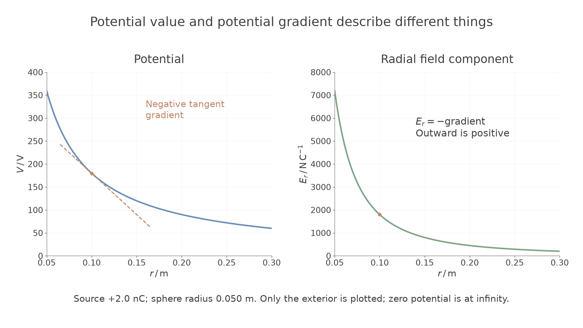
The field points in the direction of the steepest decrease of potential. On a one-dimensional potential–position graph, the signed field component is the negative gradient, not the potential value divided by the coordinate.

Potential gradient and field

E_x=-\text{gradient of the }V\text{–}x\text{ graph}

The gradient has unit $\mathrm{V\,m^{-1}}$ , equivalent to $\mathrm{N\,C^{-1}}$ . $E_x$ is the signed component along increasing position $x$ . A downward-sloping graph gives positive $E_x$ ; a rising graph gives negative $E_x$ . Use the tangent gradient for a curve. For a straight-line graph, the gradient is exactly $\Delta V/\Delta x$ .

Not on the data sheet: learn it.

The minus sign follows from energy. A positive charge released from rest accelerates along the field while losing electric potential energy, so it moves towards lower potential. A negative charge accelerates oppositely, towards higher potential, while also losing potential energy. The field direction is always defined with positive test charge.

[DIAGRAM: asset_name: Potential and field for a point charge; asset_slug: potential-field-gradients; caption: Positive-source potential decreases outwards, so its negative gradient gives an outward field; description: A potential-versus-radius curve outside a positive spherical source decreases towards zero, with a negative tangent at one marked point. An accompanying field-versus-radius curve is positive and decreases more steeply with distance. The graphs use numerical illustrative source values and begin at the sphere's surface rather than at radius zero.]
Positive-source potential decreases outwards, so its negative gradient gives an outward field

Continue this lesson.

You’re previewing NovaLearn without an account. Create a free account to read the rest.

Create free account

Last Accessed

AS foundations

AS practical skills

AS mechanics

AS waves

AS electricity

AS particles

A Level mechanics

A Level thermal physics

A Level oscillations

A Level fields and circuits

A Level quantum and nuclear physics

A Level applications

A Level practical skills

18.5 - Electric potential and potential energy

Work per unit positive charge from infinity

Field is the negative potential gradient

Continue this lesson.

Learn faster with Nova