23.2 - Random decay, activity and half-life

Unpredictable decays and fluctuating counts

A long-half-life source gives 94 counts in one minute and 111 in the next. Does the higher second count mean that the source has become more active? A detector counts individual events, and even a source with effectively constant activity over these two minutes need not give equal counts.

Radioactive decay is the spontaneous emission of ionising radiation from an unstable nucleus. Two separate ideas describe it:

Under ordinary conditions, changing a sample's temperature, pressure or chemical state does not provide a useful way to control its nuclear decay rate. Do not confuse heating an atom so that it emits light with changing its nucleus by radioactive decay.

What a counter shows

Place a detector at a fixed distance from a long-half-life source and count over equal intervals. Keep the geometry, absorber arrangement and counter settings unchanged. A sequence such as 102, 94, 111, 97, 105, 91, 109, 98 counts in successive one-minute intervals fluctuates without a steady rise or fall. Read the sequence as counts fluctuating around a mean, rather than as eight precise measurements of activity.

[DIAGRAM: asset_name: Equal intervals do not give equal counts; asset_slug: nuclear-random-counts; caption: Counts fluctuate about a mean even when the source activity changes negligibly during the observation; description: A bar chart shows 102, 94, 111, 97, 105, 91, 109 and 98 counts in eight equal one-minute intervals. A horizontal mean line at 100.875 counts is labelled about 101 counts per minute. A note states that geometry and counter settings are fixed and source half-life is much longer than eight minutes.]

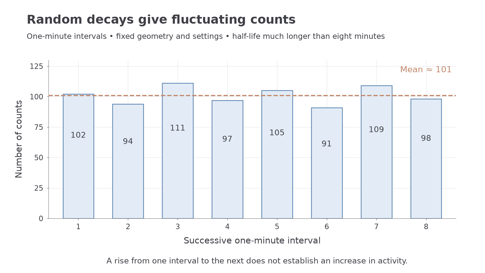
The fluctuations provide evidence for random decay. A single increase is not evidence that the source's underlying activity increased. Longer counts and repeated readings give a more reliable mean rate, although they do not make individual decays predictable. If the source changes appreciably during a long count, that count instead averages over its changing activity.

The detector also registers background radiation. Measure it with the source removed, using the same counter settings, for a sufficiently long time to obtain a useful mean. Convert both readings to the same time unit before subtraction:

This subtraction is not a supplied data-sheet formula; it is the measurement model. Background fluctuates too. A total of 600 counts in 120 seconds is $5.0\,\mathrm{s^{-1}}$. A separate background count of 120 in 300 seconds is $0.40\,\mathrm{s^{-1}}$, so the corrected source count rate is $4.6\,\mathrm{s^{-1}}$. Subtracting the raw counts 600 and 120 would mix unequal counting times.

Activity and probability per unit time

A sample with many undecayed nuclei offers many opportunities for decay. If each surviving nucleus has the same constant probability of decay per unit time, the mean number of decays per second is proportional to the number of surviving nuclei. The nucleus does not become “due” to decay because it has survived a long time.

For a sufficiently short interval $\Delta t$, the probability that a surviving nucleus decays is approximately $\lambda\Delta t$. This approximation needs $\lambda\Delta t$ much less than 1. Multiply that probability by the number of available nuclei to obtain the expected number of decays in the interval; dividing by $\Delta t$ gives the activity.

Why activity is not detector count rate

Activity counts decays in the source; corrected count rate counts registered events at the detector. Radiation is emitted in different directions, some is absorbed before reaching the detector, and not every arrival registers a count. In a fixed arrangement, write corrected count rate as $R=kA$, where $k$ is a constant detection factor for that source and apparatus. This proportionality is a measurement model, not a general supplied formula. Do not assume that $k=1$, or calculate $N$ from a detector rate without the needed detection information.

Half-life and repeated halving

Although the next individual decay cannot be timed, a large sample follows a regular statistical pattern. The same fraction of its surviving nuclei is expected to decay in each equal time interval. This produces repeated halving, rather than equal numbers disappearing in equal intervals.