2.1 - Uniform acceleration and free fall
Derive the equations for straight-line motion with constant acceleration, choose a signed equation for a journey or a falling object, and learn how an electronic fall timer can measure the acceleration of free fall. You will also use the quadratic formula when a flight time cannot be found by a single rearrangement.
Equations for constant acceleration
If a ball is released from four times the height, does it take four times as long to land? It is tempting to scale the time with the distance. But the ball gains speed as it falls, so later seconds cover more distance than earlier seconds. A model with constant acceleration lets you predict the correct scaling.
First separate the model from the world. We are describing motion along one straight line with constant acceleration. The initial velocity is , final velocity , displacement , elapsed time and acceleration . Choose a positive direction once. Velocities have unit , displacement metres, time seconds and acceleration .
From the definition of acceleration,
A constant acceleration gives a straight velocity–time line. Its area is a rectangle plus a triangle, or one trapezium. Both represent displacement.
[DIAGRAM: asset_name: The area that generates the motion equations; asset_slug: motion-constant-acceleration-area; caption: Rectangle plus triangle gives the displacement for a straight velocity-time line; description: A velocity-time line rises from u equal to 2 metres per second at zero time to v equal to 10 metres per second at 4 seconds. A blue rectangle of height 2 and width 4 lies below a pale clay triangle of height 8. The total area is 24 metres, matching the trapezium expression half times u plus v times t.]
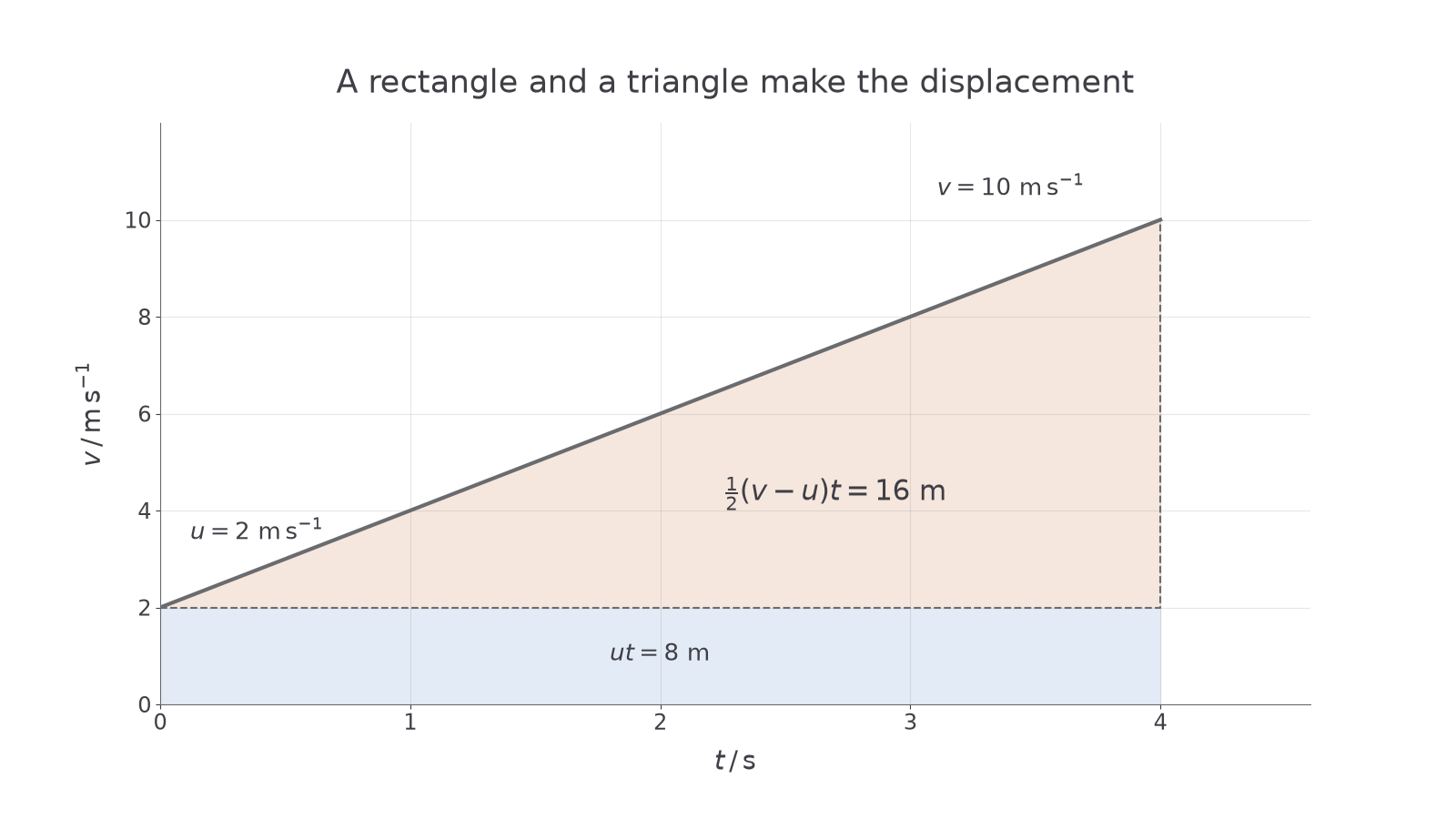
The rectangle has area ; the triangle has area . Therefore
Eliminate time instead: multiply by , then use .
These derivations are why you must not apply the equations to a changing acceleration by habit. The straight graph, and hence its simple triangular area, is part of the reasoning.
Constant-acceleration equations
Use signed displacement and velocities along one axis. The symbols and their units are defined above; acceleration must be constant during the interval.
On the data sheet.
The two supplied equations are not the entire toolkit. From their derivations you should also know , , and, by replacing with , . These three forms are not printed on the general data sheet: learn them. The equations describe signed displacement even if the object reverses direction; total distance then needs the journey split at the reversal.
Signed motion and free fall
The easiest equation is usually the one that omits a quantity you do not know and do not need. List the known signed values, identify the target and check that acceleration can be treated as constant before substituting.
Worked example 1: stopping without a time
Question. A vehicle slows uniformly from to rest over . Calculate its acceleration. Use the supplied relation .
Plan. Take forwards as positive. No time is needed.
Check. Acceleration opposes the positive velocity, so the vehicle slows down.
In free fall, gravity is the only force acting. Near Earth's surface, and over modest changes in height, the acceleration can be treated as constant and downwards. Neglect air resistance. The data sheet gives its magnitude as . If upwards is positive, , even while the object is rising. “Released from rest” means ; “thrown” does not.
For a release from rest through a downward height , choose downwards positive. The supplied equation becomes , so . Increasing by a factor of four increases the time by a factor of two. For example, ideal falls of and take about and . The larger height is covered at a greater average speed.
Some flight-time problems give a quadratic equation. Recall the mathematical tool rather than repeatedly trying numbers: if , then
The quadratic formula is not on the physics data sheet: learn it. Here capital , and are coefficients, not accelerations; their units must be consistent with the equation. Interpret both roots in the physical time interval.
Exam-style example: landing below the launch point
Question. A ball is thrown vertically upwards at from above the ground. Neglect air resistance. Determine the time before it reaches the ground. Use and .
Plan. Set the release point as zero and upwards as positive. The ground has displacement , not .
Writing the numerical equation with in seconds gives , so
The roots are and . Only the positive root lies after release.
Answer. .
Check. It takes to reach the top. The ground is below the release point, so the full flight must take longer than twice that ascent time; does.
Model limit
The constant-acceleration free-fall model fails when air resistance matters or the gravitational field changes appreciably along the path. A feather and a compact ball in air are not a fair test of the air-free prediction.
Choose signs before using the supplied relationship.
Measuring the acceleration of free fall
Timing a short fall by hand can give reaction-time uncertainty that is large compared with the fall time. An electronic release and impact switch make the start and finish events part of the apparatus instead of part of your reaction.
Clamp an electromagnet above an impact switch connected to an electronic timer. A steel ball is held at rest. Releasing it starts the timer; its first contact with the switch stops the timer. Measure from the bottom of the ball at release to the contact surface of the switch. This is the distance the ball travels before the stopping event, rather than the distance from the magnet or the ball's centre to the base.
[DIAGRAM: asset_name: An electronic free-fall measurement; asset_slug: motion-free-fall-timer; caption: Measure the ball's travel from its lower surface at release to first contact; description: A clamped electromagnet holds a steel ball above a horizontal impact switch and catching tray. A vertical dimension h starts at the bottom of the held ball and ends at the top contact surface. Dashed electrical leads connect release and impact events to a timer. A labelled stand supports the magnet.]
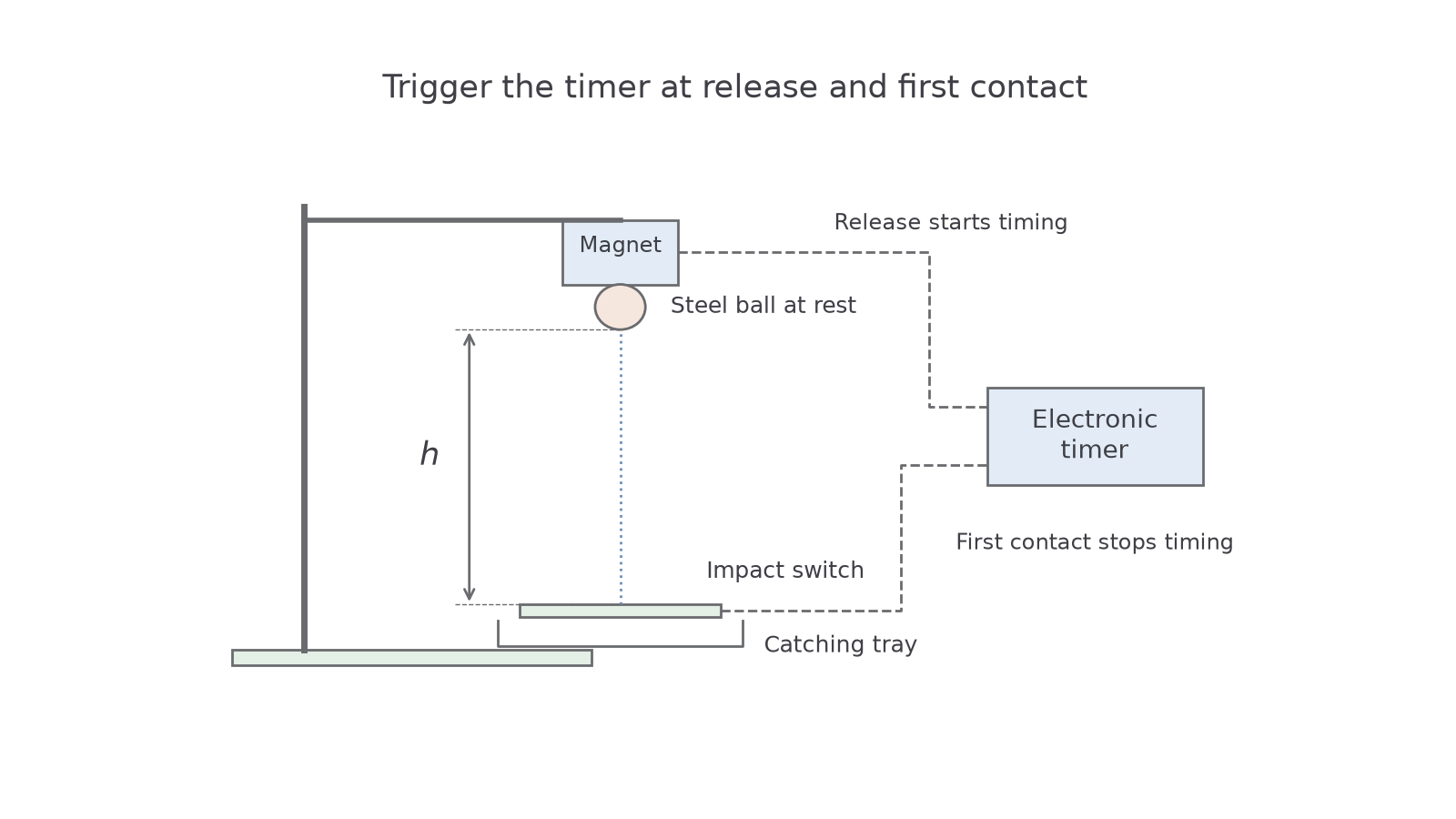
Vary the height over a useful range. At each height, repeat the release, check for unusual readings and calculate a mean time. Keep the same ball and release mechanism, and do not push the ball down. A low, clear drop zone with a catching tray reduces the risk of a ball striking feet or rolling away. Secure the stand so it cannot topple.
Practical: extracting g from a gradient
Use the following readings to practise the analysis.
| Mean | ||
|---|---|---|
| 0.20 | 0.202 | 0.0408 |
| 0.35 | 0.267 | 0.0713 |
| 0.50 | 0.319 | 0.1018 |
| 0.65 | 0.364 | 0.1325 |
From , plot vertically against horizontally. The gradient is . A best-fit line should be used; to illustrate the extraction with the extreme supplied values,
A proper experimental result includes uncertainty, not merely agreement with the expected value. Scatter, height resolution and repeat timing spread all matter.
Repeats reduce the effect of random timing variation; they do not remove a systematic delay between physical release and timer start. A constant height offset may give a non-zero intercept. A release delay can distort the height–time-squared relationship more subtly. Check how the timer is triggered and measure the actual event-to-event travel distance. Increasing the fall distance reduces relative height uncertainty, within safe limits, but a very long fall can make air resistance more significant.
Quick Recap
- Constant-acceleration equations follow from the definition of acceleration and the area under a straight velocity–time line.
- Choose one positive direction; free-fall acceleration stays downwards even while an object rises.
- Use the quadratic formula when necessary and keep only roots relevant to the physical interval.
- Electronic release/impact timing, repeated readings and a graph of against give a practical measurement of .
For an ideal release from rest, four times the height gives twice the fall time, because is proportional to .