7.04b - Average and instantaneous rates
A car can average over a journey while its speedometer shows many different speeds. Learn to distinguish an average over an interval from a rate at one instant, using chords and tangents. Then interpret the sign and units in journey, velocity and financial graphs.
Average rate from a chord
If a runner covers metres in seconds, the average speed is . That does not say the runner travels five metres in every second: the same total change can come from varying speeds.
Average rate of change
The average rate of change of from to , where , is
Graphically, it is the gradient of the chord, the straight line segment joining the two points on the curve. Not in the formula booklet: learn it.
Read both endpoint values, draw the chord when working on a graph, and use a large gradient triangle on that straight line. A triangle stretched along the curved graph would not have one constant slope. From a table or formula, calculate the same endpoint differences directly.
[DIAGRAM: asset_name: Two average rates on one distance curve; asset_slug: chord-rates; caption: Moving the second endpoint changes the chord and therefore the average rate.; description: Two panels show the distance curve d equals t squared from zero to five seconds. Chords join one one to three nine, and one one to five twenty-five, with large gradient triangles.]
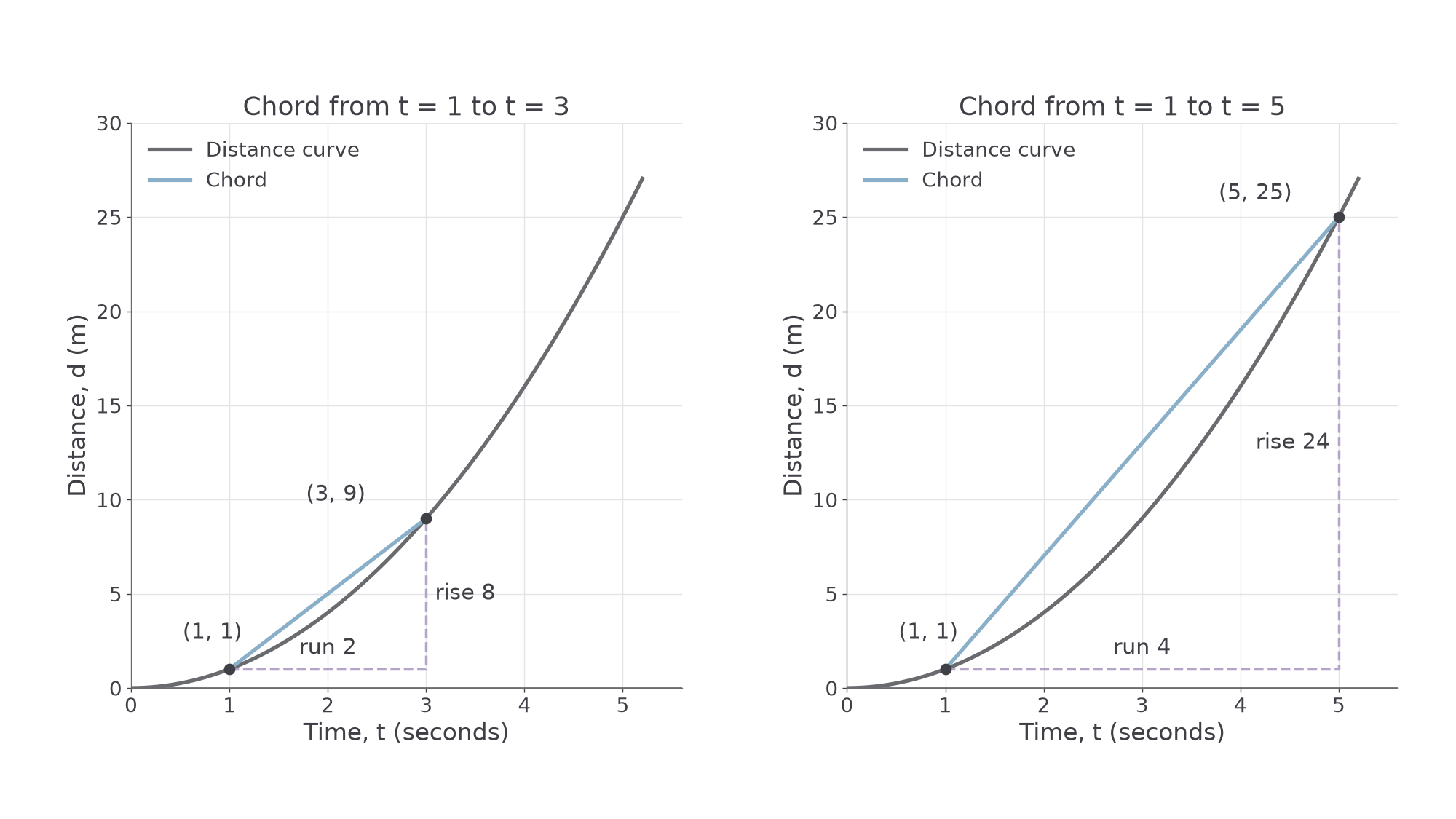
Worked example 1: average over an early interval
Question. A moving object's total distance is modelled by metres, where is in seconds. Find its average speed from to .
Plan. Calculate the two distances and divide their increase by the elapsed time.
Here means the distance at one second.
Answer. .
Check. The chord rises metres over seconds. A constant speed of four would cover the same metres in that interval.
Keep the starting time and model, but move only the ending time. The later, steeper part of the curve now contributes to the average.
Worked example 2: extending the interval
Question. For the same model , find the average speed from to .
Plan. Use the new ending distance and the new elapsed time.
Answer. .
Check. metres. The larger average fits the curve becoming steeper as time increases.
The particular model gives a useful connection. For any distinct times and , the chord gradient is
That explains both answers without inventing a constant speed along the curve. Dividing the final distance by the final time would instead average from time zero, which is a different interval.
Watch out
An average over an interval needs both endpoint changes. It is not the gradient of a tangent at the midpoint, even when the two happen to have the same numerical value for a particular curve.
Use fresh endpoints in the same model.
Instantaneous rate from a tangent
A speedometer describes the rate now, rather than over the whole journey. On a smooth distance curve, this local rate is represented by a tangent.
Instantaneous rate of change
The instantaneous rate of change at a point is the gradient of the tangent, a straight line with the curve's local direction at that point. On a total-distance-time graph this is the speed at that instant.
Place a ruler so its edge follows the curve's direction close to the required point. Draw a long straight tangent, then choose two well-separated, readable points on that line. They do not have to lie on the curve. Calculate vertical change divided by horizontal change. A small triangle magnifies reading errors, so use as much of the tangent as the grid allows.
A tangent need not remain on one side of every possible curve everywhere; what matters is the local direction at the stated point. A sharp corner has no single tangent direction, so this method assumes a smooth point. An estimate from a drawing is approximate, even if the numbers read neatly.
[DIAGRAM: asset_name: Tangents at two times; asset_slug: tangent-rates; caption: Read gradient-triangle points from the tangent line rather than from the curve.; description: Two panels show d equals t squared. At t equals two the tangent passes through one zero and four twelve. At t equals three it passes through one negative three and five twenty-one. The contact points and extended gradient triangles are marked.]
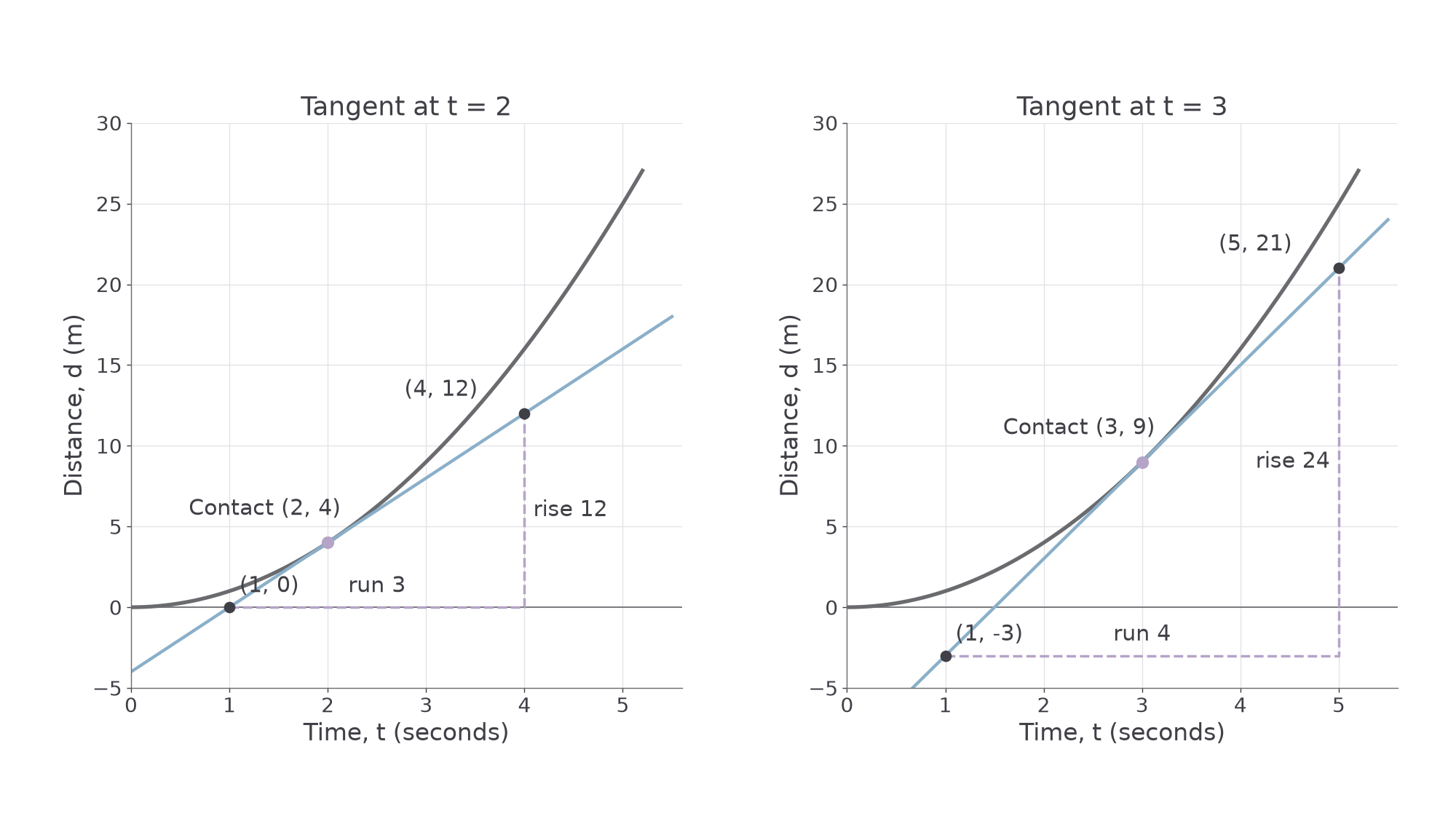
Worked example 3: estimating a local speed
Question. On the graph of , estimate the speed at . The drawn tangent has readable points and .
Plan. Use those two tangent points, not two arbitrary points on the curve.
Answer. Approximately .
Check. A short chord from to has gradient . It agrees with the local tangent estimate.
Change only the time at which the tangent touches. The same curve now has a steeper local direction.
Continue this lesson.
You’re previewing NovaLearn without an account. Create a free account to read the rest.
Create free account