12.02b, 12.03a - Histograms
A wide class can contain many observations without being the most crowded part of a distribution. In 12.02b you will construct and interpret histograms with equal and unequal intervals, using area to represent frequency. In 12.03a you will recover frequencies and estimate numerical summaries from the graph.
Frequency as an area
If one class covers twice as many possible journey times as another, should equal frequencies produce bars of equal height? A histogram answers by making the area, rather than height alone, represent frequency.
A histogram represents grouped numerical data using rectangles over the actual class intervals. Adjacent classes have touching rectangles because the horizontal scale is continuous. Their widths show class widths. The vertical axis is frequency density, the number of observations per unit of the measured variable.
The numerical area of each rectangle equals its class frequency when the height is frequency density. Class width must be positive.
This follows from rectangle area: width times height. To give a width-10 bar an area of 12, its height must be , not 12. Equal-width histograms can use heights proportional to frequencies, but the axis label and scale must state what the heights mean.
[DIAGRAM: asset_name: Equal-width histogram areas; asset_slug: equal-width-histograms; caption: Keeping frequencies fixed while halving all class widths doubles the densities and preserves the areas.; description: Two histograms. The first has intervals 0 to 10, 10 to 20 and 20 to 30 with densities 0.8, 1.2 and 0.4. The second has intervals 0 to 5, 5 to 10 and 10 to 15 with densities 1.6, 2.4 and 0.8. Areas are labelled 8, 12 and 4 in each.]
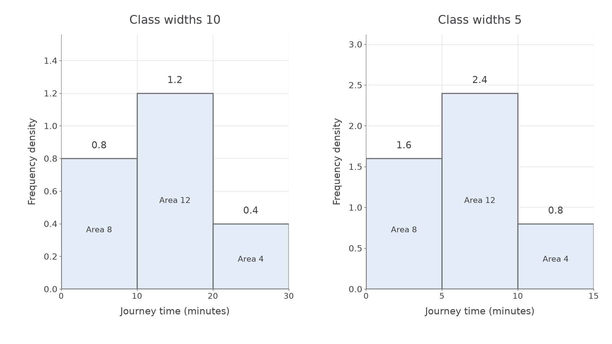
Worked example 1: constructing equal-width bars
Question. Journey-time classes , , minutes have frequencies 8, 12 and 4. Find the histogram heights.
Plan. Calculate each width, then divide each frequency by its width.
Answer. Draw touching bars over the stated intervals at heights 0.8, 1.2 and 0.4, with the vertical axis labelled frequency density.
Check. Their areas are , and , recovering all frequencies.
Now halve every class width while leaving the frequencies fixed. Only the horizontal widths change.
Worked example 2: narrower classes, equal areas
Question. Classes , , minutes have the same frequencies 8, 12 and 4. Find the heights.
Plan. Use the new common width of 5.
Answer. Heights 1.6, 2.4 and 0.8, over the new intervals.
Check. Each width has halved and height doubled, so every area is unchanged. The total frequency is still .
The surprise is useful: the same number of observations makes a taller bar when squeezed into a narrower interval. Height measures concentration.
Watch out
A histogram is not a categorical bar chart. Preserve the numerical widths and do not insert decorative gaps between adjacent classes. A genuinely empty class has zero area and should not be hidden by shifting the other bars together.
Calculate the heights for a different scale.
Unequal class intervals
When widths differ, comparing frequencies by height alone gives the wrong answer.
For each class, find upper boundary minus lower boundary separately. Draw its rectangle across that exact horizontal interval. Divide its frequency by its own width to get the height. To read a frequency, reverse the calculation by multiplying width and density.
[DIAGRAM: asset_name: Unequal intervals and changing concentration; asset_slug: unequal-width-histograms; caption: The widest bar has frequency 20, but the tallest bar depends on frequency per unit width.; description: Paired histograms have boundaries 0, 5, 15 and 35. The first has frequencies 8, 12, 20 and heights 1.6, 1.2, 1. The second changes only the middle frequency to 24, so its height becomes 2.4.]
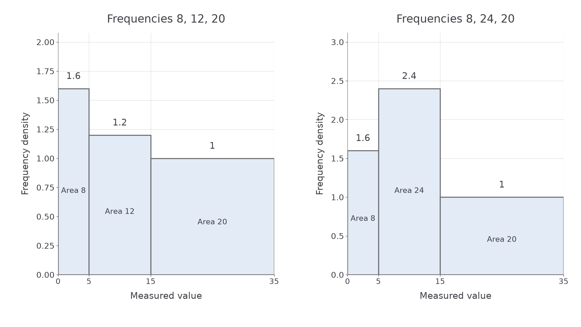
Worked example 3: a wide bar need not be tall
Question. Classes , , have frequencies 8, 12 and 20. Find the densities and identify which class has greatest frequency.
Plan. Use the three different widths, then distinguish height from area.
Answer. Heights are 1.6, 1.2 and 1. The last class has greatest frequency, 20, although the first has the tallest bar and greatest concentration per unit width.
Check. Total rectangle area is , matching .
Change only the middle frequency from 12 to 24.
Worked example 4: reconstructing a changed bar
Question. The same intervals now have frequencies 8, 24 and 20. Find the new heights and use areas to check which class has greatest frequency.
Plan. Keep widths fixed and replace the middle density.
Answer. Heights 1.6, 2.4 and 1. The middle class now has both the greatest frequency and greatest density.
Check. Its frequency doubled, so its height doubled while its width stayed 10. Total frequency rose by 12, from 40 to 52.
If the vertical scale is missing, a known class frequency can calibrate it: divide that frequency by its width to obtain its density, then use its drawn height to label the scale. After calibrating, use the same scale for every bar.
Worked example 5: calibrating an unnumbered scale
Question. On a histogram with an unnumbered vertical scale, the bar for is three equal grid steps tall and has frequency 15. The bar for is two of those grid steps tall. Find the density represented by one grid step and the second bar's frequency.
Plan. Use the known bar's area to find its density, calibrate one grid step, then recover the other area.
Answer. Each grid step represents density 1. The second frequency is 20.
Check. The second drawn area is width-by-grid units, while the first is . Their area ratio is , matching the frequency ratio.
Continue this lesson.
You’re previewing NovaLearn without an account. Create a free account to read the rest.
Create free account