12.02a, 12.03b - Time series and misleading graphs
A graph can show the right numbers and still give the wrong impression. In 12.02a you will construct and interpret time-series graphs, separating long-term trends from seasonal changes. In 12.03b you will check whether scales, labels and presentation support the claims being made.
Reading time-series graphs
If a swimming pool has more visitors in July than in January, has its popularity increased permanently? We need to know when the counts were taken, and what happened between them.
A time series records a variable at successive times. Put time on the horizontal axis in chronological order and the measured quantity, with its units, on the vertical axis. Equal horizontal distances must represent equal amounts of elapsed time. Plot each pair accurately and join successive points with straight segments. The joins help us follow change; they do not prove what happened at every unrecorded instant.
[DIAGRAM: asset_name: Constructing a monthly time series; asset_slug: monthly-time-series; caption: The time order and equal monthly spacing stay fixed when one recorded value changes.; description: Two aligned line graphs of library visits from January to April. The first has 80, 100, 90 and 120 visits. The second changes March to 110. Axes start at zero vertically and have equal monthly spacing.]
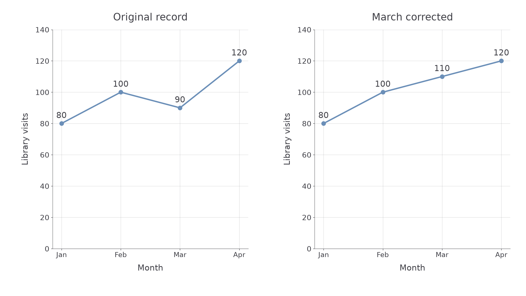
Time-series graph
A time-series graph shows how a recorded quantity varies over time. Its coordinates pair each time with its recorded value, rather than pairing two unrelated lists.
Choose a scale that uses the available space, has regular numbered intervals and includes all the observations. State whether values are daily totals, monthly totals or averages: these are different quantities.
Worked example 1: following a monthly change
Question. Library visits in January, February, March and April are 80, 100, 90 and 120. Describe how to construct the time series and find the change from February to March.
Plan. Place the months in order, plot their counts, then subtract the earlier count from the later count.
Answer. Plot the four points at equal monthly spacings on labelled axes and join them in order. Visits decreased by 10 from February to March.
Check. Adding the change to February gives , March's count. The corresponding segment slopes down.
Change only March's observation. The same subtraction now gives a different direction.
Worked example 2: a rising segment
Question. The counts are now 80, 100, 110 and 120. Give March's plotted point and the February-to-March change.
Plan. Keep the axes and other points fixed, then replace March's vertical coordinate.
Answer. Plot . Visits increased by 10.
Check. , and the new February-to-March segment slopes up.
Reading a point exactly is different from estimating between points.
Watch out
If January and April alone are recorded, their joined segment does not establish March's actual count. An intermediate reading is an estimate based on the joining rule.
Use the same time order in the next short record.
Trends and seasonal patterns
A series can rise from year to year while falling during part of every year.
The trend is the general longer-term direction: increasing, decreasing or showing no clear overall change. Seasonal variation is a pattern repeating at corresponding times in a regular cycle, such as peaks each summer. “Seasonal” can describe a regular calendar pattern, not just the four weather seasons. One isolated rise and fall does not establish repetition.
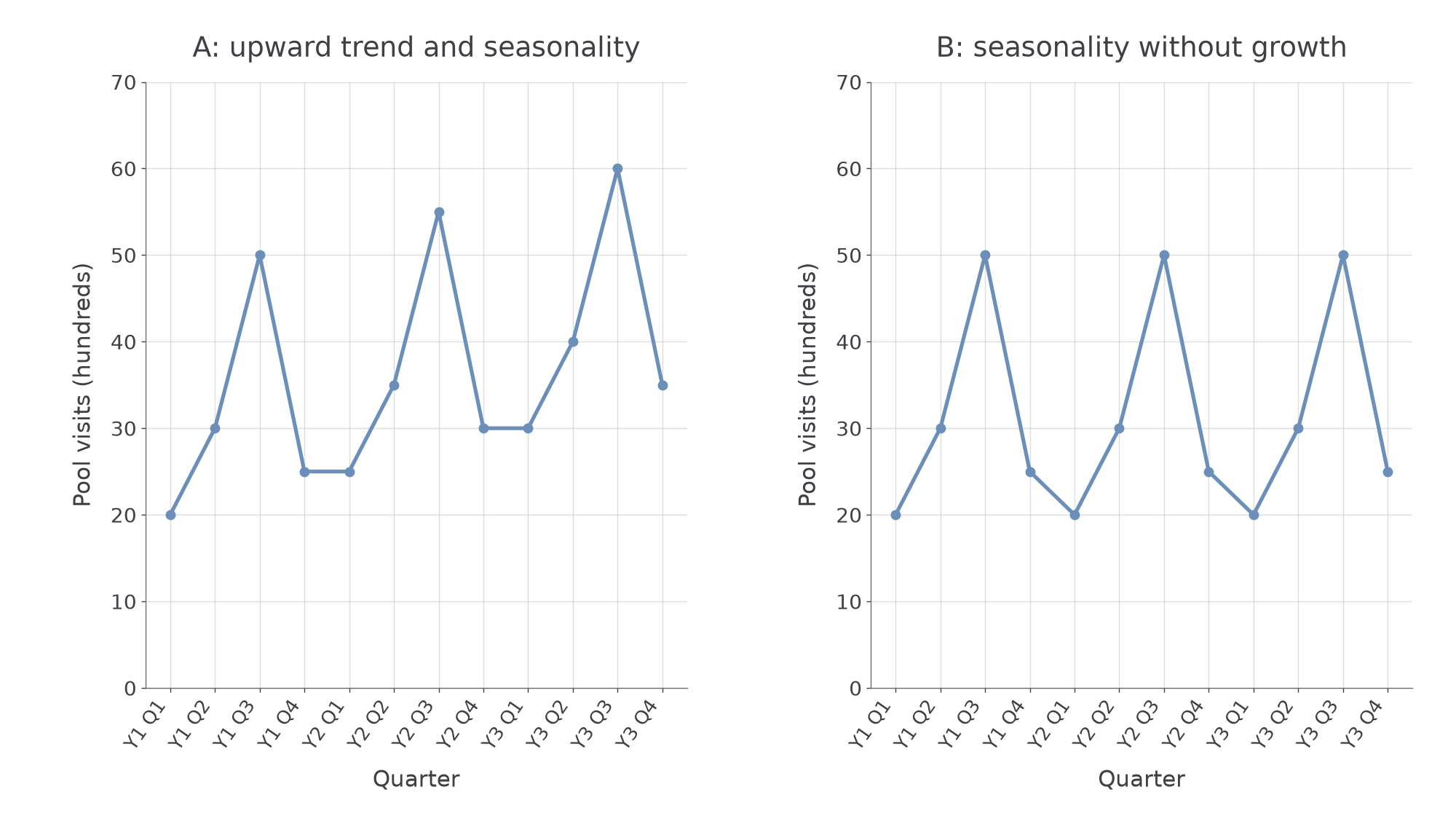
[DIAGRAM: asset_name: Trend and repeated seasonal variation; asset_slug: seasonal-patterns; caption: Compare the same quarter in successive years to see the trend beneath the repeating peaks.; description: Two quarterly time series over three years. Series A has values 20, 30, 50, 25 then 25, 35, 55, 30 then 30, 40, 60, 35. Series B repeats 20, 30, 50, 25 each year. Both peak in quarter three but only A rises between corresponding quarters.]
Worked example 3: two patterns at once
Question. Quarterly pool visits, in hundreds, are shown below. Describe the trend and seasonal pattern.
| Year | Q1 | Q2 | Q3 | Q4 |
|---|---|---|---|---|
| 1 | 20 | 30 | 50 | 25 |
| 2 | 25 | 35 | 55 | 30 |
| 3 | 30 | 40 | 60 | 35 |
Plan. Compare corresponding quarters between years, then look for repeated positions of peaks and troughs.
Answer. There is an upward trend and seasonal variation, with the highest visits in Q3 and the lowest in Q1.
Check. Q2 and Q4 also rise by five hundred visits each year. The claim uses the whole pattern, rather than just its first and last points.
Now remove only the year-to-year increases while keeping the quarterly pattern.
Continue this lesson.
You’re previewing NovaLearn without an account. Create a free account to read the rest.
Create free account