6.03e - Approximating roots by sign changes | OCR GCSE Mathematics

You can locate a solution without an exact formula for it. Use positive and negative outputs to trap a root, narrow its interval systematically and justify the number of decimal places you report. This is a Higher-tier method.

Locating a sign change

Where does the curve $y=x^3-x-5$ cross the $x$ -axis? An exact answer is awkward, but two easy substitutions can trap a crossing.

First put the equation in the form “expression equals zero”. A root is an input that makes that expression zero. For $x^3=x+5$ , rearrange to $x^3-x-5=0$ . The two sides being equal is the same as their difference being zero.

Sign-change interval

For a graph that is continuous throughout an interval, opposite signs at the endpoints guarantee at least one root between them. Continuous means the graph has no break or jump there, so it must pass through zero to get from below the axis to above it.

Polynomial graphs, including these cubics, are continuous everywhere. A sign change establishes at least one root, not necessarily exactly one. If an endpoint gives zero, that endpoint is already an exact root.

Worked example 1: trapping a cubic root

Question. Show that $x^3-x-3=0$ has a solution between $1$ and $2$ .

Plan. Substitute both endpoints into the zero-form expression and compare signs.

\begin{aligned} 1^3-1-3&=-3 &&\text{negative at }x=1\\ 2^3-2-3&=3 &&\text{positive at }x=2 \end{aligned}

Answer. The continuous cubic changes sign, so at least one solution lies between $1$ and $2$ .

Check. In the original form $x^3=x+3$ , the left side is smaller at $1$ , since $1<4$ , but larger at $2$ , since $8>5$ . This agrees with the signs.

Change only the constant. The same endpoints can still bracket a root, although the root moves.

Worked example 2: the opening equation

Question. Show that $x^3-x-5=0$ has a solution between $1$ and $2$ .

Plan. Recalculate both outputs because the constant has changed.

\begin{aligned} 1^3-1-5&=-5 &&\text{negative}\\ 2^3-2-5&=1 &&\text{positive} \end{aligned}

Answer. There is a sign change on this continuous curve, so a root lies in $1<x<2$ .

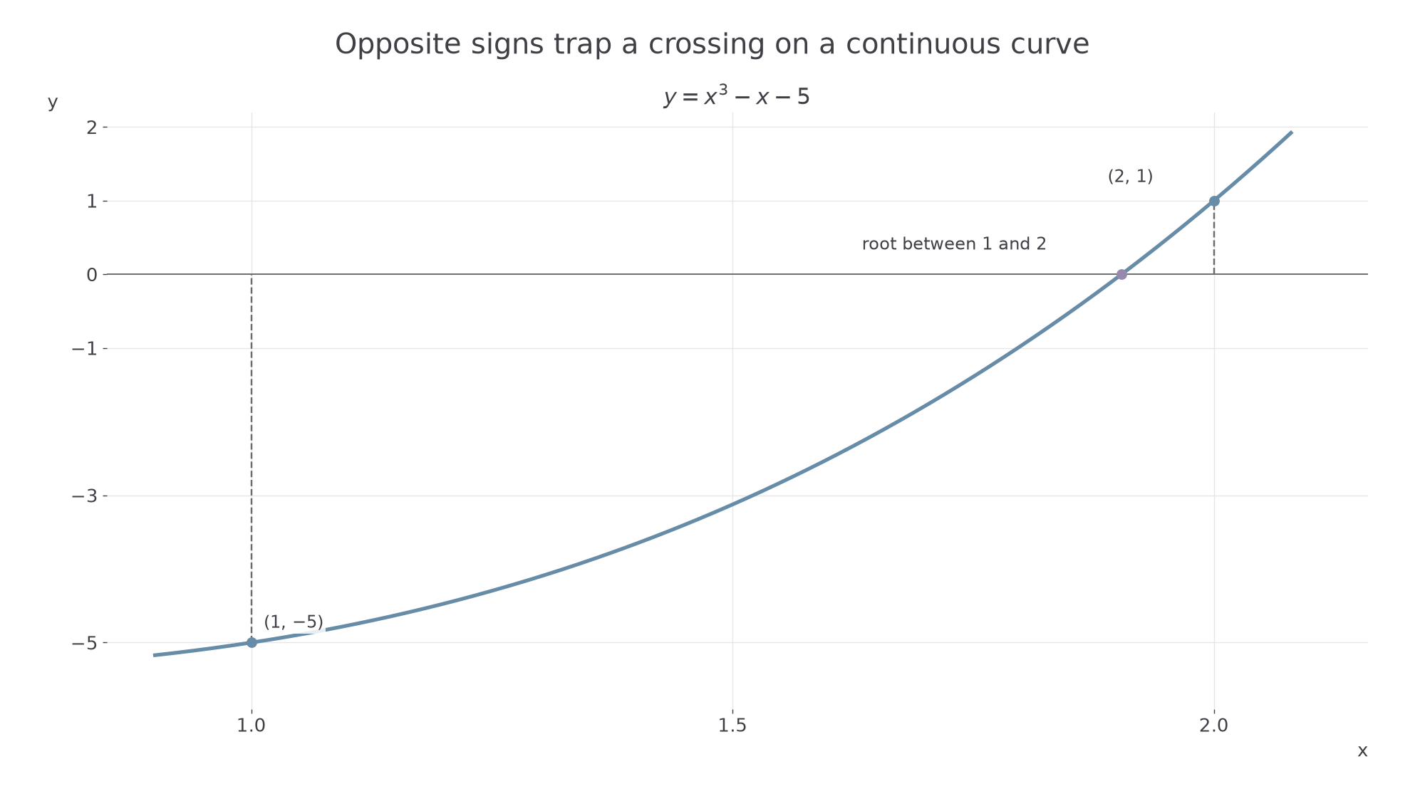
Check. The plotted curve crosses between these vertical lines. At $x=2$ , the expression is already positive but only $1$ above zero, suggesting a crossing nearer $2$ than $1$ .

The picture explains why the argument works, rather than merely showing two unrelated calculations.

[DIAGRAM: asset_name: A continuous sign change; asset_slug: sign-change-bracket; caption: The continuous cubic must cross zero between a negative output and a positive output.; description: The graph y equals x cubed minus x minus five is shown near x one to two. Points one comma negative five and two comma one are labelled, with vertical guides to the x-axis and a crossing between them.]
The continuous cubic must cross zero between a negative output and a positive output.

Watch out

Opposite signs alone are insufficient if the graph breaks inside the interval. For $y=1/x$ , the outputs at $-1$ and $1$ have opposite signs, but the graph is undefined at zero and never equals zero. Conversely, equal endpoint signs do not rule out a root: $y=x^2$ is positive at $-1$ and $1$ , yet equals zero between them.

Show both evaluations and explain their signs when asked to show that a solution lies in an interval.

Narrowing a root interval

Once you have a sign-change interval, choose another input inside it and keep the smaller interval whose endpoints have opposite signs.

Two useful choices are decimal search, testing tenths then hundredths and so on, and interval bisection, repeatedly testing the midpoint. Either is systematic. You need not memorise a particular named algorithm: choose sensible trials and show how their signs narrow the interval.

Keep the input beside each output. Otherwise a list of positive and negative numbers does not tell the reader where the root lies. Retain enough calculator digits to decide the sign reliably; do not round a tiny nonzero output to zero.

Worked example 3: a decimal search

Question. Narrow the root of $x^3-x-5=0$ to an interval of width $0.01$ .

Plan. Search in tenths inside $(1,2)$ , then hundredths inside the final tenth.

\begin{aligned} 1.8^3-1.8-5&=-0.968 &&\text{negative}\\ 1.9^3-1.9-5&=-0.041 &&\text{negative}\\ 2^3-2-5&=1 &&\text{positive}\\ 1.91^3-1.91-5&=0.057871 &&\text{positive} \end{aligned}

Answer. The outputs at $1.90$ and $1.91$ have opposite signs, trapping a root in $1.90<x<1.91$ .

Check. $1.91-1.90=0.01$ , and direct evaluation of both retained endpoints gives opposite signs. The interval is inside the original one.

Keep the same equation but change the search choice to midpoints. Each successful step halves the interval width.

Worked example 4: bisecting an interval

Question. Starting from $1.9<x<2$ , make two bisection steps for $x^3-x-5=0$ .

Plan. Average the endpoints, evaluate there, then retain opposite signs.

\begin{aligned} \tfrac{1.9+2}{2}&=1.95 &&\text{first midpoint}\\ 1.95^3-1.95-5&=0.464875 &&\text{keep }(1.9,1.95)\\ \tfrac{1.9+1.95}{2}&=1.925 &&\text{second midpoint}\\ 1.925^3-1.925-5&=0.208328125 &&\text{keep }(1.9,1.925) \end{aligned}

Answer. After two steps, $1.9<x<1.925$ .

Check. The lower output remains $-0.041$ and the upper output is positive. The width is $0.025=0.1/4$ , as expected after two halvings.

Continue this lesson.

You’re previewing NovaLearn without an account. Create a free account to read the rest.

Create free account

Last Accessed

Number

Algebra

Ratio and proportion

Geometry and measures

Graphs and functions

Probability

Statistics

6.03e - Approximating roots by sign changes

Locating a sign change

Narrowing a root interval

Continue this lesson.

Learn faster with Nova