11.01b, 11.01c - Estimating probability from experiments
If a coin shows heads twelve times in twenty tosses, is its chance of heads really ? In 11.01b, organise repeated outcomes in tables and frequency trees. In 11.01c, use relative frequency to estimate probability, and explain why more trials can improve evidence while still allowing variation.
Recording repeated outcomes
To learn from an experiment, record every trial once under a clear outcome category. Categories should not overlap, and together they should include all possible results. Their frequencies must add to the number of trials.
A frequency is a count. For repeated pairs of coin tosses, the categories , , and keep the order of the tosses. The table below records sixty trials; each trial consists of two tosses.
| Outcome | ||||
|---|---|---|---|---|
| Frequency |
Worked example 1: analysing a frequency table
Question. Use the table to find the total number of trials and the number whose first toss was heads.
Plan. Add all categories for the total, then only the categories starting with .
Answer. There were trials, and had heads first.
Check. The categories starting with tails give . The two first-toss groups sum to .
Now change only the representation of the same results. A frequency tree splits a total into groups, then splits each group again. The numbers are counts, not probabilities. At every split, the child counts add to their parent count.
[DIAGRAM: asset_name: A frequency tree for repeated pairs of tosses; asset_slug: experiment-frequency-tree; caption: Each pair of branch counts adds to the total from which it splits.; description: A frequency tree starts at sixty trials. First heads and first tails each have count thirty. The heads group splits into second heads fourteen and second tails sixteen. The tails group splits into second heads eighteen and second tails twelve.]
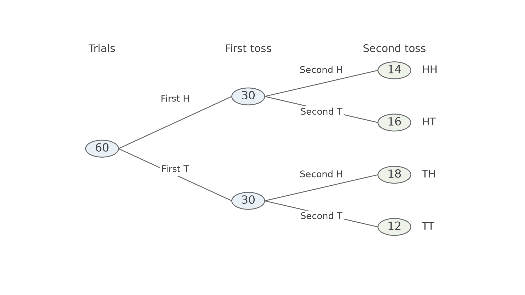
Worked example 2: completing a frequency tree
Question. For these same sixty trials, a partly completed tree gives first-heads count , , and . Find the first-tails count, and .
Plan. Subtract known child counts from their parent totals.
Answer. First tails: ; ; .
Check. The four final counts total , and each pair of end branches sums to its first-toss group of thirty.
In either representation, the count describes first heads and second heads. To count second heads regardless of the first toss, add and : . Follow the meaning of the branches, rather than combining numbers simply because they are near each other on the page.
Watch out
A branch count of thirty is not a probability of thirty. Keep counts in a frequency tree; divide by the appropriate trial total only when estimating a probability.
Complete a fresh set of counts textually.
Relative frequency as an estimate
A theoretical probability comes from a model, such as equally likely faces on a fair dice. An experimental estimate comes from what actually happened. We use the event's share of all trials, called its relative frequency.
Relative frequency
For a positive number of trials,
Use this fraction or decimal as an estimate of probability when the trials are relevant to the future experiment. With no trials, this estimate is undefined.
Not in the formula booklet: learn it.
Suppose a machine's operating conditions stay the same. Its recorded failure share can help predict a future failure count. If the machine is repaired or the material changes, the old share may no longer be a useful probability estimate. The assumption about comparable conditions matters as much as the arithmetic.
Worked example 3: estimating and predicting
Question. In trials of a spinner, it lands on red times. Estimate the probability of red and predict the red count in another comparable spins.
Plan. Divide the red frequency by the trial total, then use this estimate in the expected-count calculation.
The hat indicates an estimate.
Answer. Estimated probability ; predicted count .
Check. . The new prediction has the same red share as the observed results.
Change only the total number of recorded spins while keeping the red frequency thirty-two. A count without its denominator cannot describe a probability.
Worked example 4: the denominator changes the estimate
Question. A different record has red results in spins. Estimate the probability of red and predict the red count in comparable spins.
Plan. Use the new denominator, then scale the resulting share.
Answer. Estimated probability ; predicted count .
Check. The same thirty-two successes now occur in twice as many trials, so the relative frequency and predicted count are both halved.
Continue this lesson.
You’re previewing NovaLearn without an account. Create a free account to read the rest.
Create free account