12.02b, 12.03a - Cumulative frequency and box plots
How can you find the middle half of a distribution without listing every observation? In 12.02b you will build and read cumulative-frequency graphs. In 12.03a you will estimate medians and quartiles, construct box plots and compare distributions using their median and interquartile range.
Constructing cumulative frequency
Suppose task times are grouped into intervals. To find how many people finished before 20 minutes, add every relevant earlier class, not just the class ending at 20.
Cumulative frequency is a running total of frequencies. A “less than” cumulative-frequency graph pairs each upper class boundary with the number below that boundary. Start at the first lower boundary with cumulative frequency zero. For intervals written with an included upper boundary, the running totals instead count values up to and including it; follow the table's inequalities consistently.
Cumulative-frequency graph
A cumulative-frequency graph plots running frequency vertically against the measured variable horizontally. It cannot decrease, and its final height is the total frequency.
Use labelled numerical scales. Plot the boundary points, then join them with a sensible increasing curve or straight segments as appropriate. We will use straight segments between known boundary points, making the within-class estimation rule explicit. The actual distribution between them is unknown; a curve does not restore the hidden observations.
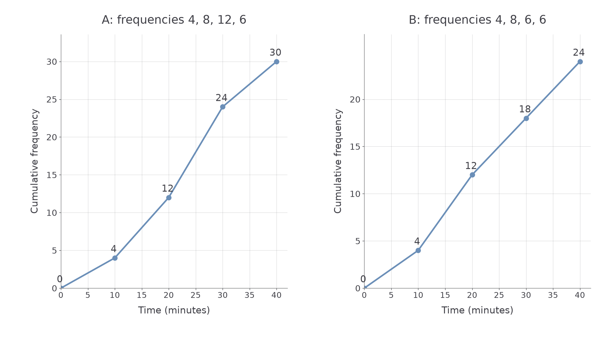
[DIAGRAM: asset_name: Constructing two cumulative-frequency graphs; asset_slug: cumulative-construction; caption: Plot the running total at each upper boundary and begin at the lower boundary with zero.; description: Two line graphs use time boundaries 0, 10, 20, 30 and 40 minutes. A has cumulative frequencies 0, 4, 12, 24 and 30. B changes the third class frequency from 12 to 6 and has cumulative frequencies 0, 4, 12, 18 and 24. All plotted boundary points are marked.]
Worked example 1: boundaries and running totals
Question. Construct the cumulative-frequency points for task times with frequencies 4, 8, 12 and 6 in intervals , , , .
Plan. Add each frequency to the preceding total and attach the result to its upper boundary.
Answer. Plot the five points on axes labelled time in minutes and cumulative frequency, then join them in order using increasing segments.
Check. Consecutive vertical increases are 4, 8, 12 and 6, reconstructing the original frequencies. The final height is 30, the total.
Change only the third class frequency from 12 to 6.
Worked example 2: later totals change together
Question. Find the new points when the frequencies are 4, 8, 6 and 6 over the same intervals.
Plan. Keep the first two running totals, then add the changed frequency and everything after it.
Answer. The points at 30 and 40 minutes become and ; the earlier points stay fixed.
Check. The total fell by 6, from 30 to 24. Both later running totals fell by 6, although only one class frequency changed.
An empty class produces a horizontal section. A steep section means many observations per unit of the measured variable; compare steepness with care when class widths differ.
Watch out
Plot at upper boundaries, not class midpoints. Midpoints represent classes when estimating a mean; upper boundaries mark the point by which all that class's frequency has accumulated.
Use the boundaries and running totals to specify the graph's points.
Estimating medians and quartiles
The graph turns a position in the ordered data into an estimated value of the variable.
The median splits the distribution in half. The lower quartile marks approximately one quarter of the observations, and the upper quartile approximately three quarters. Their difference is the interquartile range, the spread of the middle half. For a grouped graph with total frequency , use these cumulative-frequency levels:
Move horizontally from the chosen frequency level to the graph, then vertically down to read the variable. These are grouped graph estimates, not an instruction to locate the -th individual observation in a known raw list.
Between plotted boundaries, straight-line interpolation assumes that observations are spread evenly across the interval. A fraction of the class frequency then corresponds to the same fraction of its width.
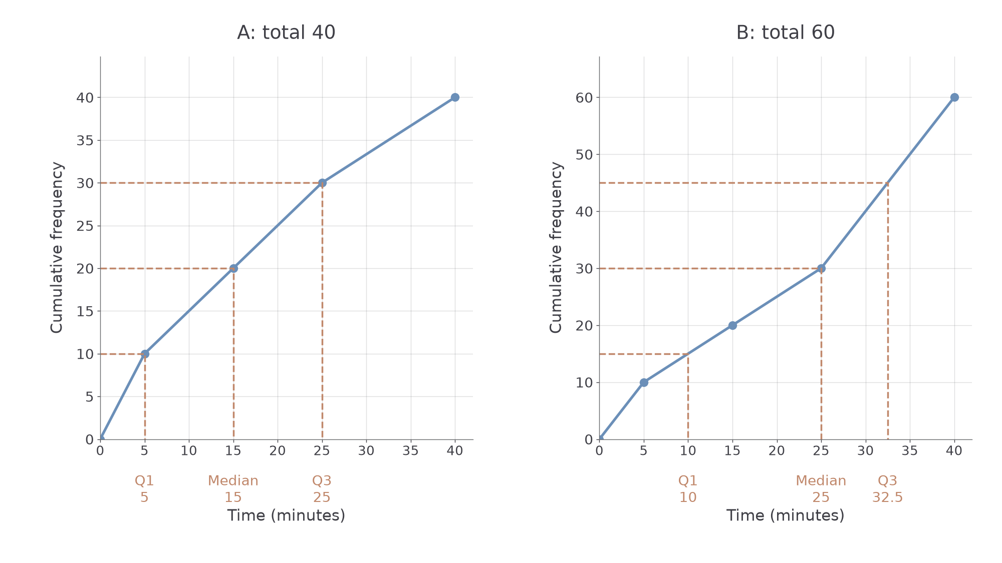
[DIAGRAM: asset_name: Reading quartiles from cumulative frequency; asset_slug: cumulative-quartiles; caption: Use one-quarter, one-half and three-quarters of the final frequency, then read across and down.; description: Two cumulative-frequency graphs have horizontal boundaries 0, 5, 15, 25 and 40. A has cumulative values 0, 10, 20, 30 and 40 with quartile guides at counts 10, 20 and 30. B has cumulative values 0, 10, 20, 30 and 60 with guides at counts 15, 30 and 45.]
Worked example 3: reading three positions
Question. Graph A joins . Estimate its median, quartiles and IQR.
Plan. Read the final total, calculate the three count levels and trace across and down.
Answer. Estimated quartiles 5 and 25, median 15 and IQR 20.
Check. The cumulative count rises from 10 to 30 between 5 and 25. This is 20 of 40 observations, the middle half.
Change only the last class frequency from 10 to 30. Its final cumulative height becomes 60, so the quartile count levels must change too.
Worked example 4: interpolating between boundaries
Question. Graph B joins . Make the same estimates.
Plan. Use levels 15, 30 and 45, interpolating on the stated straight segments.
Answer. Estimated quartiles 10 and 32.5, median 25 and IQR 22.5.
Check. At 10 the interpolated count is 15; at 32.5 it is 45. Their difference is 30, half the new total of 60.
You can also estimate how many observations lie below or above a stated value. Start at that value on the horizontal axis, move up to the graph and across to the cumulative-frequency axis to read the count below it. Subtract this from the total to estimate the count at or above the threshold. For continuous measurements, the interpolation model assigns no separate frequency to a single exact value, so this also estimates the count above it.
Worked example 5: reading how many finish later
Question. Graph B joins . Estimate how many task times are below 30 minutes and how many are above 30 minutes.
Plan. Read the running count at 30, then subtract it from the final total of 60.
Answer. About 40 times are below 30 minutes and about 20 are above it.
Check. The two estimated groups total . Thirty minutes is one third of the way from 25 to 40, so the running count is one third of the way from 30 to 60.
Change only the threshold from 30 to 35 minutes, staying on the same straight segment.
Continue this lesson.
You’re previewing NovaLearn without an account. Create a free account to read the rest.
Create free account