5.1.1(h) - Initial rates, continuous monitoring and colorimetry
Rate experiments turn a visible change into numerical evidence. In this lesson you will learn how chemists measure reaction rates using initial-rate methods, continuous monitoring, and colorimetry, then how those methods feed into the rate graphs and rate equations used elsewhere in 5.1.1. The emphasis is practical: what to measure, why the method works, what must be controlled, and how OCR-style questions expect you to use the data.
Two rate methods
A rate experiment must measure a quantity that changes as the reaction proceeds. That quantity might be concentration, gas volume, mass, absorbance, or the time taken for a fixed visible change. The chosen quantity is useful only if it can be linked reliably to the amount of reactant used up or product formed.
There are two main approaches in this specification point.
Initial rates method
An initial rates method measures the rate at, or very close to, the start of a reaction. Separate experiments are run with different starting concentrations, and one initial rate is found for each mixture.
Continuous monitoring
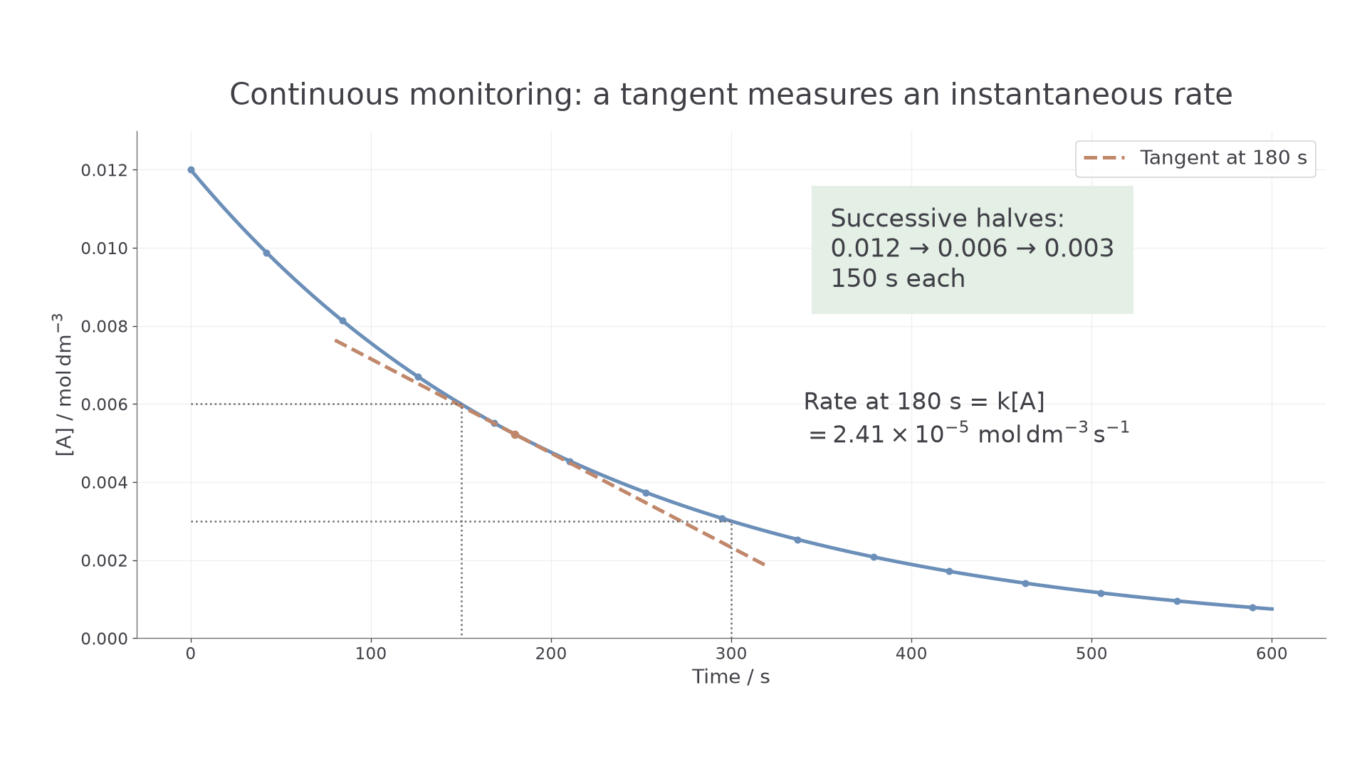
Continuous monitoring follows one reaction mixture through time by recording repeated or logged measurements. A graph of the changing quantity against time is then used to find rates from gradients.
The practical difference is important. In an initial-rate experiment, each run is deliberately short or uses only the first part of the reaction, so the concentrations have not changed much. In a continuous-monitoring experiment, the whole curve matters: the gradient is steep at first, then usually becomes less steep as reactants are used up.
The unit of rate depends on what is being measured. For reaction-rate calculations in concentration terms, OCR commonly uses:
Rate from concentration change
If concentration is in and time is in seconds, the rate unit is .
Initial rates give one early rate from each separate mixture; continuous monitoring gives a whole time course from one mixture.
Initial rates in practice
The initial rates method is useful when you want to compare how changing a starting concentration changes the rate. You keep all other variables constant, run the reaction several times, and determine the rate close to .
One route is to collect early concentration-time data and draw a tangent at the start of the curve. The gradient of that tangent is the initial rate. Another route is a clock reaction. In a clock reaction, the time is measured until a fixed visible change occurs, such as the appearance of a colour or enough sulfur precipitate to obscure a mark.
For a clock reaction, the key assumption is that the same small amount of reaction has happened when the visible endpoint is reached each time. If that fixed amount is small, then:
Clock-rate comparison
This is a comparison method, not a new definition of rate. It is most reliable when the endpoint is reached quickly, because the reaction mixture is then still close to its initial concentrations.
Worked example
A thiosulfate-acid clock experiment is repeated at two different thiosulfate ion concentrations. The same total volume, acid concentration and temperature are used each time.
| Experiment | Initial / | Time for endpoint / | / |
|---|---|---|---|
| 1 | 0.0500 | 80.0 | 0.0125 |
| 2 | 0.100 | 40.0 | 0.0250 |
When doubles, doubles. Since is proportional to the initial rate for this clock method, the initial rate doubles. That evidence is consistent with first order with respect to thiosulfate ions, although the full order-deduction method belongs with the rate-equation lessons.
Good initial-rate method design is mostly about fairness. Keep the total volume constant by adding water where needed, use the same temperature, use the same endpoint, mix in the same way, and start timing at the same point in the method. Repeat readings help identify an anomalous endpoint time.
The common mistake is to treat as an exact concentration rate in . It is normally an initial-rate measure for comparison unless the fixed concentration change at the endpoint is known.
Continuous monitoring
Continuous monitoring records how a physical quantity changes during the reaction. The method is chosen to match the reaction:
- collect gas in a gas syringe or over water if a gas is produced
- measure mass loss if a gas escapes from the reaction vessel
- use a colorimeter if a coloured reactant or product changes concentration
The rate at a particular time is found from the gradient of the curve at that time. For a concentration-time graph of a reactant, the gradient is negative because the reactant concentration is falling. The rate of disappearance is usually reported as a positive value, so take the magnitude of the gradient.
[DIAGRAM: asset_name: Lesson 5.1.1h: Initial rates, continuous monitoring and colorimetry - diagram 01; asset_slug: 05_01_01c_initial_rates_continuous_monitoring_and_colorimetry__diagram_01; recommended_method: matplotlib; description: Concentration-time graph for a monitored coloured reactant showing data points, a smooth curve, a tangent used to find rate at a chosen time, and two equal half-life intervals as evidence for first-order behaviour.]
Worked example
A concentration-time graph for a reactant has a tangent drawn at . Two convenient points on the tangent are:
The tangent gradient is:
The rate of disappearance of the reactant at is therefore:
OCR rate-graph questions often reward the evidence as much as the final value. State that you used a tangent at the required time, show the two coordinate values used, and include units.
Collecting a gas without losing the start
Place a measured acid volume in a conical flask connected by a gas-tight bung and delivery tube to a freely moving, securely clamped gas syringe. Keep the solid reactant separate until the apparatus is sealed, then mix and start the timer together. Record syringe volume at short regular intervals, keeping temperature and solid surface area constant. Use a syringe with enough capacity; never block the outlet or restrain the plunger. A leak under-records volume and a sticking plunger distorts the early gradient.
[DIAGRAM: asset_name: Continuous gas monitoring apparatus; asset_slug: h432_511h_gas_monitoring; recommended_method: drawn_chem; description: Sealed conical flask and gas delivery tube lead to a horizontal clamped gas syringe with free plunger; time-volume data supply a tangent rate.]
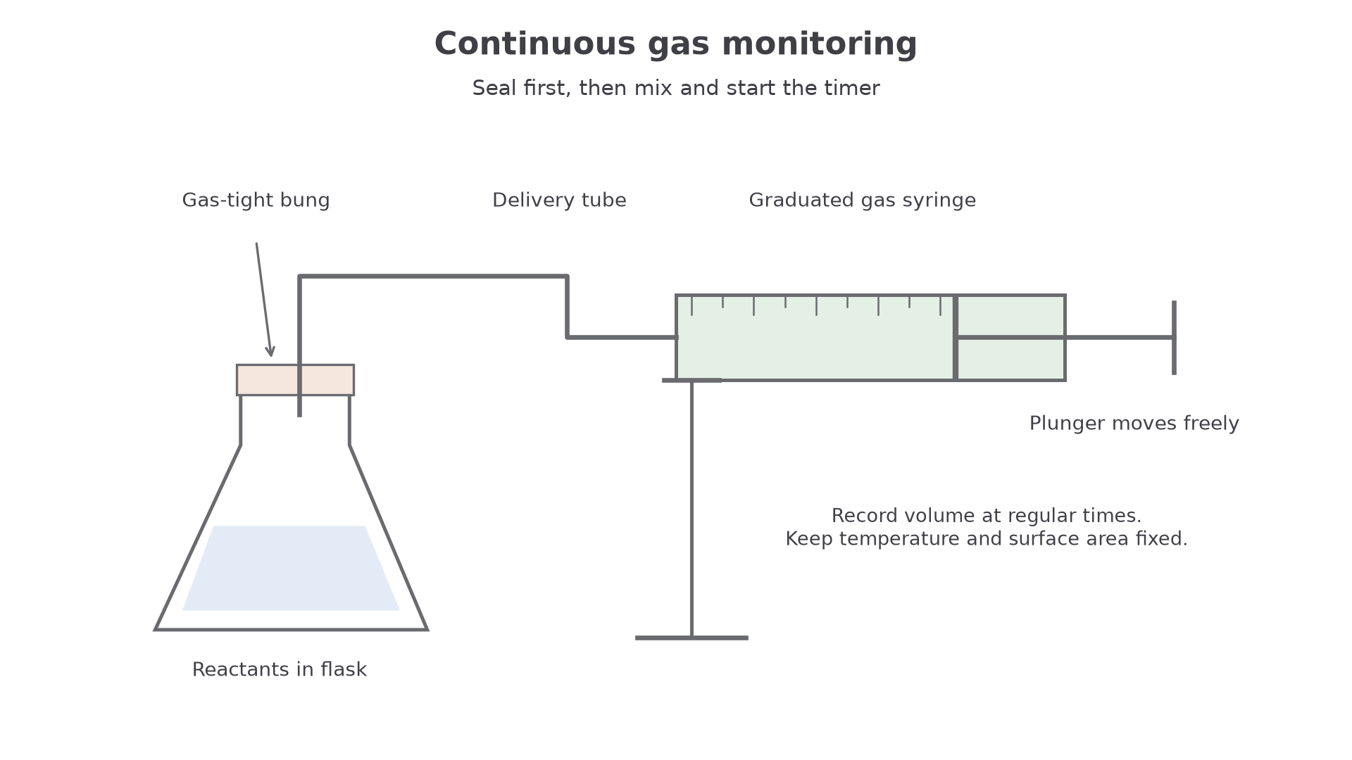
A volume gradient measures gas volume per unit time. At a molar gas volume of 24.0 , divide a rate in by 24000 to obtain . To obtain a solution concentration change per second, also use the reacting mole ratio and divide by solution volume in .
Continue this lesson.
You’re previewing NovaLearn without an account. Create a free account to read the rest.
Create free account