1.1.3 - Analysis, graphs and significant figures
This lesson is about turning practical results into evidence. You will learn how to process qualitative and quantitative results, choose sensible significant figures, draw and interpret graphs, and use gradients, intercepts and tangents to support a valid conclusion.
From Results to Conclusions
Raw observations do not become chemistry until you interpret them. A strong practical conclusion does three things: it identifies the pattern, supports it with evidence, and stays within what the data can actually show.
Valid Conclusion
A valid conclusion is a statement supported by the experimental evidence and consistent with the method used. It should not claim more precision or certainty than the data justify.
Qualitative results describe what is observed: colour changes, precipitates, gas formation, temperature changes or no visible change. Quantitative results use numbers: mass, volume, time, temperature, pH, concentration, rate or calculated values. Both types need careful processing.
Good analysis follows a sequence:
- Check what was measured and what units were used.
- Process repeated or calculated data consistently.
- Identify the pattern, trend or comparison.
- Link the pattern to the chemistry being tested.
- Write a conclusion that mentions the evidence.
Worked reasoning: a student tests three metal carbonates with dilute acid. All three fizz, and the gas turns limewater cloudy. The valid qualitative conclusion is that carbon dioxide was produced in each reaction, supporting carbonate ions being present. It would be too broad to conclude that the samples were pure carbonates unless the method had tested purity.
Processing Quantitative Data
Processing data means changing raw measurements into values that answer the practical question. This may involve differences, means, ratios, percentages, rates or formula substitution. The mathematics should be shown clearly enough that another chemist can follow it.
For repeated measurements, do not average values blindly. First check whether a value is anomalous in the context of the set. If a value is clearly inconsistent and there is a practical reason to doubt it, flag it and process the remaining comparable repeats. Detailed judgement about why it happened belongs in evaluation.
Worked example: calculating a rate from volume data
A reaction produces 42.0 cm³ of gas in the first 60.0 s.
The unit comes from the calculation: volume divided by time. This is an average rate over the first 60.0 s, not necessarily the instantaneous rate at exactly 60.0 s.
Quantitative conclusions should quote the processed value and its meaning. "The reaction is faster" is weak. "The reaction at 40 °C has a mean gas-production rate of 0.700 cm³ s⁻¹, which is double the rate at 30 °C" is much stronger if the data support it.
For three comparable clock times of 31.2, 31.6 and 31.4 s, the mean time is . Its reciprocal is , a relative rate measure, not a concentration change per second. It represents initial-rate comparisons only when the fixed endpoint corresponds to the same small amount of chemical change and reactant concentrations change little before it. Keep the raw times, state the processing choice, and do not mix reciprocal mean time with the mean of reciprocal times without explanation.
Ratios test a specific claim. If doubling concentration changes the measured rate from 0.24 to 0.48 cm³ s⁻¹, the ratio is 2.0, consistent with proportionality for those measurements. One pair does not prove that relationship across an untested range; inspect all points and their uncertainty.
Read mathematical relationships
A symbol states a relationship; changing it can change the chemical claim. Use for equality: . Use and for smaller and larger values: a 20 s clock time is less than a 40 s clock time, but its reciprocal is larger. The signs and mean much smaller and much larger; for example, a 0.01 g uncertainty is much smaller than a 10.00 g mass, but not necessarily negligible for a 0.02 g sample.
The proportionality sign means a constant factor relates two quantities under stated conditions. For a fixed small clock endpoint, relative initial rate is proportional to ; doubling halves that rate measure. It does not say that the numerical chemical rate in mol dm⁻³ s⁻¹ equals . The symbol can mean approximately or “of the order of” in an estimate; make the intended meaning clear and use when explicitly rounding a number, for example .
The reversible-reaction sign indicates that a chemical reaction can proceed in both directions. It is not an equals sign between numerical quantities, and it does not say that the amounts on the two sides are equal. Detailed equilibrium reasoning is taught later; here the skill is reading the statement correctly.
Significant Figures
Significant figures communicate the precision of a number. They are not decoration: too few significant figures lose useful information, while too many suggest more precision than the experiment supports.
Significant Figures
Significant figures are the meaningful digits in a measured or calculated value. Leading zeros are not significant; zeros between non-zero digits are significant; final zeros after a decimal point are significant.
Examples:
| Value | Significant figures | Why |
|---|---|---|
| 0.00450 | 3 | 4, 5 and the final 0 are meaningful |
| 12.0 | 3 | the decimal zero shows measured precision |
| 100 | ambiguous | it may mean 1, 2 or 3 significant figures unless written more clearly |
| 1.00 × 10² | 3 | standard form makes the precision clear |
In calculations, keep extra digits during working and round the final answer at the end. If a question asks for a specific number of significant figures, follow the instruction. If it does not, give a sensible number that matches the data, commonly the same number of significant figures as the least precise measured value used in the calculation.
Worked example: using sensible significant figures
A student calculates:
The input values are all given to three significant figures, so a sensible final answer is:
Do not round early. If 0.245 had been rounded to 0.25 at the start, the final answer would be less accurate.
For addition or subtraction, compare the decimal-place resolution, not simply the number of significant figures. A burette difference retains two decimal places. An exact count or stoichiometric coefficient does not limit the precision: dividing a sum by exactly three repeats does not restrict a mean to one significant figure. Uncertainty, where supplied, is a stronger guide than blindly counting digits.
Plotting Suitable Graphs
A graph is useful only if another person can read what has been plotted. Axes must be selected, labelled and scaled properly.
For a suitable graph:
- put the independent variable on the x-axis where possible
- put the dependent variable on the y-axis
- label each axis with the quantity and unit, such as time / s or volume of gas / cm³
- choose scales that use most of the graph area and are easy to read
- plot points accurately
- draw a best-fit straight line or smooth curve when appropriate
- do not force a line through the origin unless the chemistry and data justify it
Worked reasoning: choosing axes
If the experiment changes temperature and measures rate, temperature is the independent variable and belongs on the x-axis. Rate is the dependent variable and belongs on the y-axis. An axis label such as rate is incomplete; use the measured or calculated quantity and unit, for example rate / cm³ s⁻¹.
Gradients and Intercepts
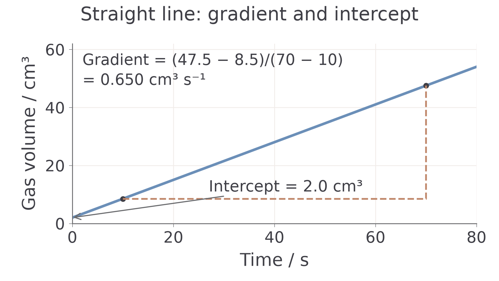
For a straight-line graph, the gradient measures how much the y-value changes for each unit change in x.
Gradient
Use two well-separated points on the best-fit line, not necessarily two raw data points. Draw or imagine a large gradient triangle so small reading errors matter less. The unit of the gradient is the y-axis unit divided by the x-axis unit.
Worked example: gradient from a straight line
The straight-line diagram below has a best-fit line passing through (10 s, 8.5 cm³) and (70 s, 47.5 cm³).
The intercept is where a line crosses an axis. In chemistry, an intercept can have a meaning only if the graph and model support it. For example, an intercept on a calibration graph may represent a background reading, but an intercept should not be overinterpreted without context.
A straight line can also be written as , where is its gradient and is its y-intercept. If the origin is outside the drawn grid, calculate using a point on the best-fit line. For the gas-volume example above, .
Worked example: reading an intercept
A calibration graph has absorbance on the y-axis and concentration on the x-axis. The best-fit line crosses the y-axis at 0.020 absorbance units. The y-intercept is therefore 0.020 absorbance units. It may represent a small blank or background reading only if the method supports that interpretation; otherwise, report it as a graph feature rather than proof of a cause.
[DIAGRAM: asset_name: Gradient and intercept of a straight best-fit line; asset_slug: c01_straight_line_gradient; recommended_method: drawn_chem; description: A gas-volume best-fit line has gradient 0.650 cm³ s⁻¹ and intercept 2.0 cm³; a large gradient triangle uses points at 10 s and 70 s.]
Tangents and instantaneous rates
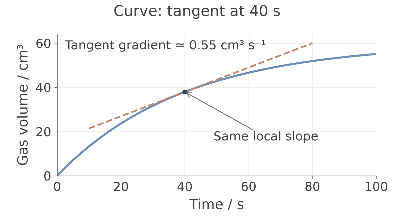
Curved graphs need a different method. If a curve shows how a quantity changes with time, its gradient gives the instantaneous rate of change at that time. Draw a tangent with the same local slope as the curve at the chosen point, then calculate the tangent gradient using two well-separated points on that line. For a decreasing reactant concentration, the gradient is negative; the positive rate of disappearance is the magnitude of that gradient.
Worked example: tangent gradient
The tangent in the diagram below touches the curve at 40 s. Two well-separated points on that tangent are approximately (20 s, 26.9 cm³) and (80 s, 60.0 cm³).
That value is the estimated instantaneous rate at 40 s. It is not the average rate from 20 s to 80 s for the curve; those two points are on the tangent line used for measurement.
A tangent can cross the curve elsewhere; what matters is matching its local slope at the stated time. The two points used in the gradient calculation belong to the tangent and need not be measured data points.
[DIAGRAM: asset_name: Local tangent on a gas-volume curve; asset_slug: c01_curve_tangent; recommended_method: drawn_chem; description: A tangent at 40 s has the same local slope as the gas-volume curve; its gradient is approximately 0.55 cm³ s⁻¹.]
Quick Recap
- Support conclusions with processed evidence and state what the results cannot establish.
- Use consistent units, keep unrounded working and report a justified final precision.
- A mean rate uses a whole interval; an instantaneous rate uses the local gradient.
- Label graph axes with quantities and units, use readable scales and an appropriate best fit.
- Calculate gradients with well-separated points on the fitted line or tangent, and give the gradient unit.
- Interpret proportional relationships and intercepts in their chemical context.