5.1.1(d)-(g) - Concentration-time and rate-concentration graphs

Two graph families

Before reading any graph, ask what the axes mean. OCR uses two related graph families in this topic, but they answer different questions.

A concentration-time graph shows how the concentration of one reactant changes during one experiment. It is usually produced by continuous monitoring: for example, measuring colour intensity, gas volume, mass, pH or another property as the reaction proceeds, then converting the readings into concentration where needed.

A rate-concentration graph shows how the initial rate changes when the initial concentration of one reactant is changed across separate experiments. The other conditions, especially temperature and the concentrations of other reactants, must be controlled so the graph is evidence for the order with respect to that one reactant.

Concentration-time shape and rate

These shape deductions assume the rate depends only on the plotted reactant, or that other rate-affecting reactants remain effectively constant. On a concentration-time graph for a reactant, the line normally slopes down because reactant concentration falls as the reaction proceeds. The rate of disappearance of the reactant is the magnitude of the gradient:

The minus sign is there because the reactant concentration decreases, so the gradient itself is negative. In answers, rate is usually given as a positive value with units such as $\,\mathrm{mol} \,\mathrm{dm}^{-3} \,\mathrm{s}^{-1}$ or $\,\mathrm{mol} \,\mathrm{dm}^{-3} \,\mathrm{min}^{-1}$.

OCR expects two concentration-time shape deductions in this split:

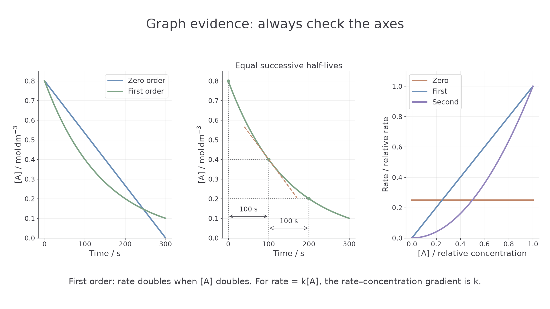
• Zero order with respect to the reactant: the concentration-time graph is a straight decreasing line. The gradient is constant, so the rate stays constant even as that reactant is used up.
• First order with respect to the reactant: the concentration-time graph is a decreasing curve that becomes less steep. As concentration falls, the rate falls.

For a curved concentration-time graph, the rate at a particular time is found from the gradient of a tangent at that time. Choose two well-spaced points on the tangent, calculate change in concentration / change in time, then give the positive magnitude for a reactant.

Worked example

A tangent to a reactant concentration-time curve at $t = 80 \,\mathrm{s}$ passes through $(40 \,\mathrm{s}, 0.92 \,\mathrm{mol} \,\mathrm{dm}^{-3})$ and $(130 \,\mathrm{s}, 0.47 \,\mathrm{mol} \,\mathrm{dm}^{-3})$.

Gradient of tangent:

The reactant is disappearing, so:

First-order half-life

Successive halving intervals let you test whether the falling concentration follows first-order kinetics.

For a first-order reaction, successive half-lives are constant. This means it takes the same time for $[A]$ to fall from $0.80$ to $0.40 \,\mathrm{mol} \,\mathrm{dm}^{-3}$, from $0.40$ to $0.20 \,\mathrm{mol} \,\mathrm{dm}^{-3}$, and from $0.20$ to $0.10 \,\mathrm{mol} \,\mathrm{dm}^{-3}$, within experimental uncertainty.

That constancy is powerful evidence. On a concentration-time graph, you can mark one horizontal line at an initial concentration, another at half that concentration, and read the time gap between them. Repeat for the next halving. If the times are the same or very close, OCR expects the conclusion that the reaction is first order with respect to that reactant.

Be careful with the wording: a first-order graph is not just "curved". The strongest concentration-time evidence is constant half-life, or equivalent tangent evidence showing that when concentration halves, the rate halves.

Worked example

A reactant concentration falls as follows on a graph:

• $0.120 \,\mathrm{mol} \,\mathrm{dm}^{-3}$ at $0 \,\mathrm{s}$
• $0.060 \,\mathrm{mol} \,\mathrm{dm}^{-3}$ at $150 \,\mathrm{s}$
• $0.030 \,\mathrm{mol} \,\mathrm{dm}^{-3}$ at $300 \,\mathrm{s}$

Each halving takes $150 \,\mathrm{s}$, so the half-life is constant. The reaction is first order with respect to that reactant.

Read each half-life as a time interval, not as the time coordinate at the later concentration. For example, if $[A]$ is 0.160 at 40 s, 0.080 at 130 s and 0.040 $\mathrm{mol\,dm^{-3}}$ at 220 s, the halving intervals are $130-40=90$ s and $220-130=90$ s. They are not 130 s and 220 s. The constant interval supports first-order behaviour even though the first reading is not at time zero.

The diagram compares mathematically generated curves. Equal horizontal time intervals correspond to successive halvings; the dashed tangent is local to one time, not a line joining two points on the curve.

[DIAGRAM: asset_name: Rate graphs and half-life; asset_slug: 05_01_01b_concentration_time_graphs_half_life_and_rate_concentration_graphs__diagram_01; recommended_method: matplotlib; description: Three panels compare zero-order and first-order concentration-time curves, exact constant half-life intervals with a tangent, and zero/first/second-order rate-concentration graphs.]