SH1, SH3 - Confidence intervals with known variance
Construct symmetric confidence intervals for a normal population mean when its variance is known. You will connect the interval to the sampling distribution, interpret confidence correctly and use a constructed or given interval to assess a proposed mean.
Constructing a normal-mean interval
A sample mean is 102, but how wide a range should we report for the population mean? An estimate without its uncertainty can look more precise than the data justify.
Suppose 25 independent measurements are randomly sampled from a normal population whose standard deviation is known to be 10. The sample mean has standard deviation . This is the standard error of the mean, describing how much sample means vary, rather than how much individual observations vary.
For a standard normal variable, the central 95% lies between approximately and . Applying these rounded boundaries to the mean and rearranging gives
The random quantity in this second line is the pair of endpoints, both based on the random sample.
Known-variance confidence interval
For independent random observations from , with known , a symmetric confidence interval for is
where . The margin of error (half-width) is .
The standardised normal sampling pivot is in the formula booklet; this rearranged interval formula is not printed separately. Familiar normal critical values appear in the infinite-degrees-of-freedom row of its t table; other quantiles can be found with an inverse-normal calculator function.
Normality makes this sampling result exact for any positive sample size; a large-sample threshold is not required when the population really is normal and is known. Unknown requires a different treatment taught next.
Worked example 1: a 95% interval
Question. For , and known , construct a 95% confidence interval for the normal population mean.
Plan. Use the normal standard error and put 2.5% outside each endpoint.
Answer. The 95% interval is .
Check. Its midpoint is 102. Each endpoint is 3.92 from the midpoint, corresponding to standard errors.
Keep the sample and known standard deviation fixed; change only the confidence level to 99%. Greater coverage requires a wider interval.
Worked example 2: a higher confidence level
Question. Construct the 99% confidence interval from the same data, using .
Plan. Use the same standard error and allow 0.5% in each tail.
Answer. The interval is , or to two decimal places.
Check. Its width is , exceeding the earlier width . Their ratio equals the ratio of the critical values, as only confidence changed.
Watch out
Wrong: use 0.95 as the cumulative probability for a symmetric 95% interval. Correct: use . Also distinguish known variance 100 from its standard deviation 10.
Confidence describes the procedure
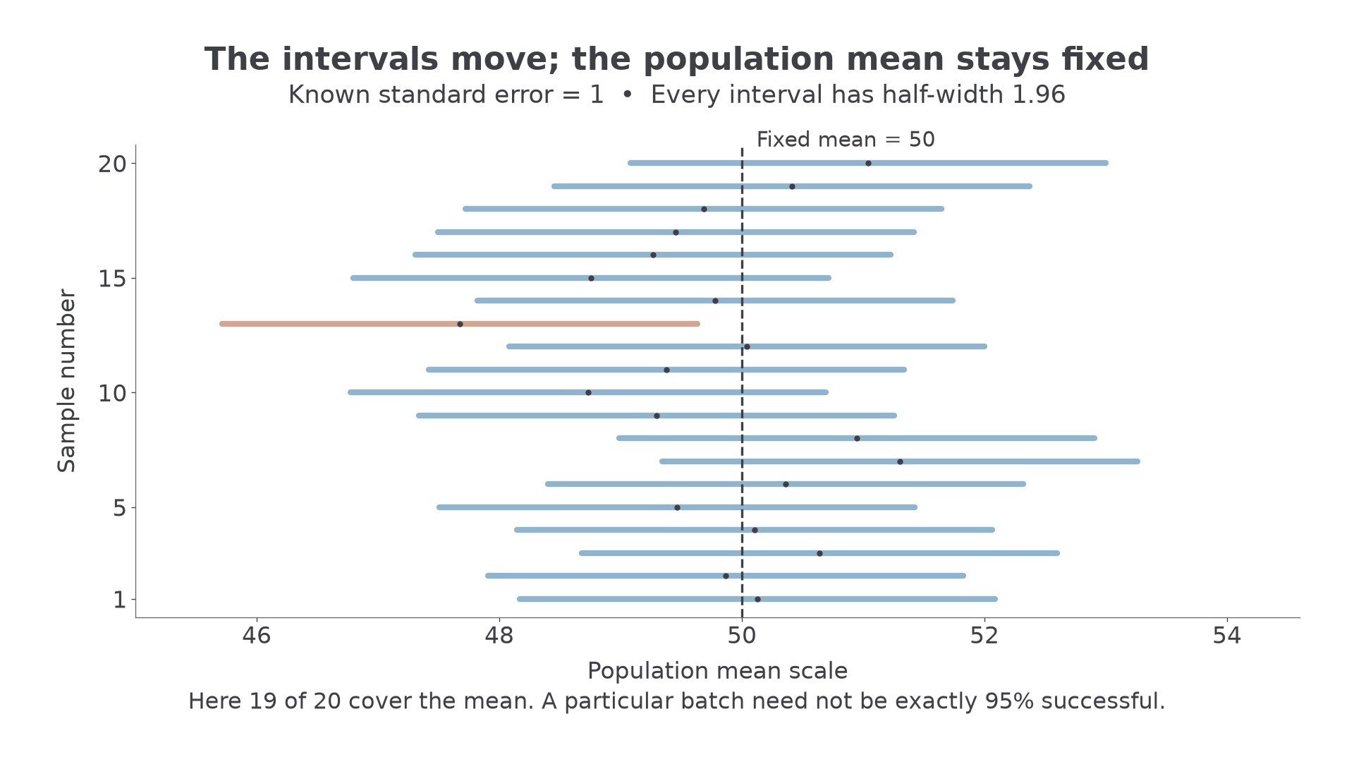
Imagine repeatedly taking independent samples of the same size from the same population, and constructing a 95% interval each time. Sample means change, so interval locations change. With known and fixed , their widths stay the same.
95% confidence
A 95% confidence procedure produces intervals that contain the fixed population mean in 95% of repeated samples under the stated assumptions. The percentage describes the procedure's long-run coverage.
[DIAGRAM: asset_name: Repeated confidence intervals; asset_slug: aqa7367-confidence-coverage; caption: Intervals move with the sample mean while the population mean stays fixed; description: Twenty illustrative 95 percent intervals with known standard error one are plotted horizontally against sample number. All have half-width 1.96. A vertical dashed line marks the fixed population mean 50. Nineteen intervals cross the line and one does not. The missed interval is clay and covering intervals are blue. A note says a particular batch need not contain exactly 95 percent successful intervals.]
Continue this lesson.
You’re previewing NovaLearn without an account. Create a free account to read the rest.
Create free account