J3 - Improved Euler’s method | AQA A-Level Further Mathematics

A slope at the middle of an interval can estimate the change across the whole interval. You will use AQA’s two-step improved Euler recurrence, obtain its missing starting value with Euler’s method, and compare estimates at the same endpoint. Careful indexing matters as much as the arithmetic.

Use the two-step central recurrence

For $\mathrm{d}y/\mathrm{d}x=y$ , $y(0)=1$ , how can a slope at $x=0.1$ help estimate the height at $x=0.2$ ? Instead of taking a short tangent step from the latest point, estimate the change from $x=0$ to $x=0.2$ using the slope halfway across.

Suppose $x_{r-1},x_r,x_{r+1}$ are equally spaced, with gap $h$ . The whole interval from $x_{r-1}$ to $x_{r+1}$ has width $2h$ . For a smooth solution and small nonzero $|h|$ , its chord gradient is approximated by the derivative at the middle:

\frac{y(x_{r+1})-y(x_{r-1})}{2h}\approx y'(x_r) =f\bigl(x_r,y(x_r)\bigr).

Rearrange, then replace the unknown exact solution heights by numerical estimates.

Two-step improved Euler method

For $\mathrm{d}y/\mathrm{d}x=f(x,y)$ ,

y_{r+1}=y_{r-1}+2h f(x_r,y_r),\qquad x_{r+1}=x_r+h, \qquad r\ge1.

This is the improved Euler formula supplied on page 9 of the examination formula booklet. It needs two starting heights, $y_0$ and $y_1$ , on an equally spaced grid. The derivative must be defined at every evaluation point.

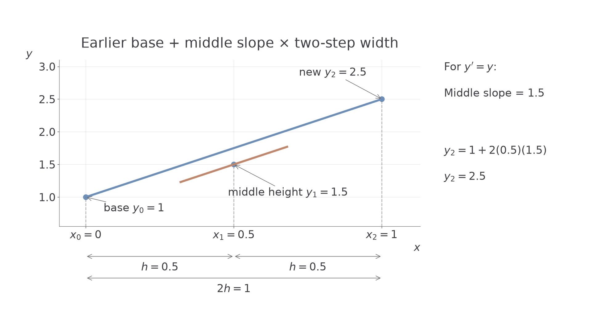
The base height and the gradient come from different rows: start at $y_{r-1}$ , but evaluate the gradient at $(x_r,y_r)$ . The factor $2h$ is the distance from the base point to the new point. The slope point lies halfway between them.

[DIAGRAM: asset_name: A central slope bridges two steps; asset_slug: aqa7367-improved-euler; caption: Start from the earlier height and use the middle slope across a width of two h; description: A coordinate diagram for y prime equals y shows points at x equals zero, 0.5 and one with heights one, 1.5 and 2.5. A blue bridge from (0,1) to (1,2.5) has slope 1.5. A parallel clay segment through (0.5,1.5) shows the middle-row slope. Below the axis, two adjacent widths h equals 0.5 and their total 2h equals one are marked. Labels distinguish the earlier base height, middle height and new height.]
Start from the earlier height and use the middle slope across a width of two h

Worked example 1: bridge successive pairs of steps

Question. For $y'=y$ , take $h=0.1$ , $(x_0,y_0)=(0,1)$ , and the supplied estimate $y_1=1.1$ at $x_1=0.1$ . Use the two-step method to find $y_2$ and $y_3$ .

Plan. For each new height, use the height two rows earlier plus $2h$ times the intervening gradient.

\begin{aligned} y_2&=y_0+0.2y_1=1+0.2(1.1)=1.22\\ y_3&=y_1+0.2y_2=1.1+0.2(1.22)=1.344. \end{aligned}

Answer. $y(0.2)\approx1.22$ and $y(0.3)\approx1.344$ .

Check. Across the first bridge, $(1.22-1)/0.2=1.1$ , exactly the middle gradient. Independently, the exact solution $e^x$ gives approximately $1.221403$ and $1.349859$ ; neither numerical value should be labelled exact.

Now change only the grid spacing, with a corresponding supplied starting estimate. Keeping the factor $2h$ visible prevents a missing factor of two.

Worked example 2: a wider grid

Question. For $y'=y$ , take $h=0.2$ , $y_0=1$ at $x_0=0$ , and the supplied estimate $y_1=1.2$ at $x_1=0.2$ . Find $y_2$ and $y_3$ .

Plan. The bridge width is now $0.4$ , although consecutive grid positions differ by $0.2$ .

\begin{aligned} y_2&=1+0.4(1.2)=1.48 &&x_2=0.4\\ y_3&=1.2+0.4(1.48)=1.792 &&x_3=0.6. \end{aligned}

Answer. $y(0.4)\approx1.48$ and $y(0.6)\approx1.792$ .

Check. The exact values $e^{0.4}\approx1.491825$ and $e^{0.6}\approx1.822119$ are nearby. These endpoints differ from those in Worked example 1, so the two final heights alone do not compare the methods’ accuracy at a common point.

For an equation $y'=f(x)$ with no height dependence, each bridge adds $2h f(x_r)$ . That is precisely one midpoint rectangle for the integral of the derivative across the bridge: another connection between differentiation and quadrature.

Watch out

Wrong: $y_2=y_1+2h f(x_1,y_1)$ . That adds a two-step change to the wrong base height. Correct: $y_2=y_0+2h f(x_1,y_1)$ .

Practise with a changed starting height.

Start the recurrence with an Euler step

One initial condition provides $y_0$ , but the central recurrence cannot yet calculate $y_1$ : it would require an unavailable $y_{-1}$ .

Use ordinary Euler once to produce the second starting height, unless a different starting value or procedure is explicitly supplied:

y_1=y_0+h f(x_0,y_0).

Then switch to the two-step recurrence, beginning at $r=1$ . Keep the original $y_0$ ; it is still needed to calculate $y_2$ . Store two previous heights rather than overwriting one in place.

The Euler starting value is an approximation, so it influences later results. A supplied more accurate $y_1$ can change the answer even if every subsequent central step is identical. This does not license replacing the requested start in an examination task.

Worked example 3: initialise, then switch methods

Question. For $y'=x+y$ , $y(0)=1$ , take $h=0.1$ . Use Euler once, then the two-step improved Euler method to estimate $y(0.3)$ .

Plan. Calculate $y_1$ by a one-step tangent update, then obtain $y_2,y_3$ from two-step bridges.

\begin{aligned} y_1&=1+0.1(0+1)=1.1 &&\text{Euler start}\\ y_2&=1+0.2(0.1+1.1)=1.24 &&\text{base }y_0\\ y_3&=1.1+0.2(0.2+1.24)=1.388 &&\text{base }y_1. \end{aligned}

Answer. $y(0.3)\approx1.388$ .

Check. The exact function $2e^x-x-1$ satisfies the equation and initial condition. At $x=0.3$ it gives approximately $1.399718$ , confirming a small approximation error rather than equality.

Change only the starting procedure: suppose a more accurate $y_1$ has been supplied. The central recurrence stays the same.

Continue this lesson.

You’re previewing NovaLearn without an account. Create a free account to read the rest.

Create free account

Last Accessed

Core Pure

Mechanics

Statistics

Discrete Mathematics

J3 - Improved Euler’s method

Use the two-step central recurrence

Start the recurrence with an Euler step

Continue this lesson.

Learn faster with Nova