G3 - Areas inside polar curves
Polar areas are built from thin sectors rather than vertical strips. You will derive the area formula, choose bounds from the actual tracing, and calculate regions inside or between curves. Careful sketches will help you avoid counting a region twice or subtracting the wrong radii.
Area from thin sectors
How can you measure the overlap of the circles and without finding Cartesian strip heights? Use the rays from their shared pole as the slices.
For a circle of fixed radius , a sector with angle in radians occupies the fraction of the circle. Its area is therefore
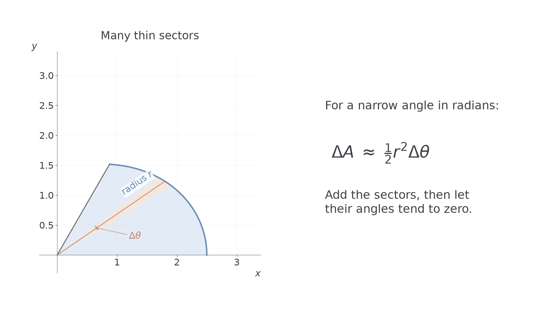
For a varying radius , a very narrow slice is approximately such a sector. If is continuous, the smallest and largest radii on the slice bound its area between two sector areas. As the slice widths tend to zero, those approximations lead to the same integral. This explains both the square of the radius and the factor .
[DIAGRAM: asset_name: Building polar area from sectors; asset_slug: aqa7367-polar-area-sectors; caption: A narrow angular slice has area approaching one half r squared times its angle; description: A shaded radial region is divided conceptually into thin sectors, with one narrow sector highlighted. The radius r and small angle delta theta are labelled. The neighbouring panel gives delta A approximately one half r squared delta theta and explains adding sectors as their angles shrink to zero.]
Polar area
For a nonnegative, continuous radius , the area swept from the pole to the curve between rays and is
provided the chosen sweep covers the required region once, with no repeated interior. Piecewise-continuous boundaries can be split into suitable pieces. Use radians and .
This polar-area formula is supplied in the formula booklet, on page 8. Selecting the region and bounds remains your task.
Unlike Cartesian area under a graph, the radius is not a signed height. This formula measures areas of radial sectors. Repeated tracing repeats their areas; squaring an inadmissible negative radius does not make its angle admissible under a nonnegative-radius convention.
Worked example 1: a constant-radius sector
Question. Find the area between the pole and , for .
Plan. Integrate half the squared radius across the given angular width.
Answer. square units.
Check. This sector is one sixth of a circle of area , giving .
Keep the angle interval and replace the constant radius by . The sector formula still works, but the changing radius must be squared before integration.
Worked example 2: a changing-radius sector
Question. Find the area between the pole and , for , with .
Plan. Square the full radius and use .
Answer. square units.
Check. The curve is the circle of radius 1 centred at . Its upper semicircle has area . The omitted cap beyond ray is a sector of central angle minus a triangle, area . Subtracting it gives the same result. The answer is also smaller than Worked example 1, since every radius here is at most 2.
The identity turns a squared cosine into terms whose antiderivatives you know. Keep the chain factor when integrating .
Watch out
Wrong: when . Squaring the entire radius gives , not .
Change only the radius scale in a new problem.
Selecting bounds and counting once
The bounds describe a sweep of rays, not horizontal coordinates. Before integrating, identify the region, find its boundary rays, and follow the curve through the proposed interval. An endpoint can be a given ray, a pole crossing found from , or a nonzero intersection found by equating radii.
For , traces the whole circle once. The smaller interval traces its upper half. Integrating over that half and doubling is valid; integrating over the whole circle and then doubling is not.
A petal such as , , starts at the pole, reaches radius 3 at , then returns to the pole. Those two zero-radius bounds enclose one petal. Over a larger interval, solve the sign restriction again and count the distinct petals; do not integrate blindly across forbidden angles.
For the cardioid , the radius stays nonnegative. A sweep traces its complete boundary once, returning through a cusp at . Although two parameter values label the starting boundary point, that shared endpoint has zero area; it does not duplicate an interior region.
Worked example 3: the complete cardioid
Question. Find the total area enclosed by , with .
Plan. Use one full tracing from 0 to , then expand the square and replace .
Answer. square units.
Check. Over a full turn, the average values of and are zero. Thus the expanded integrand has mean 3 over width , confirming . The region fits inside the radius-4 circle of area .
Keep the curve and change only the requested region to its upper half. Symmetry should halve the result, rather than require a new formula.
Worked example 4: half of the same cardioid
Question. Find the area enclosed by above the initial line.
Plan. Trace the upper arc with and integrate once.
Answer. square units.
Check. Reflection in the initial line preserves the cardioid, so its upper and lower areas are equal. Twice this result agrees with the independently computed total in Worked example 3.
If signed radii are explicitly allowed, over traces its circle twice: the negative-radius half-turn repeats the positive-radius points. Its integral then gives twice the circle's area. Under the nonnegative-radius convention those negative-radius angles are excluded instead. Either way, tracing must be settled before interpreting the integral as a geometric area.
Continue this lesson.
You’re previewing NovaLearn without an account. Create a free account to read the rest.
Create free account