SA6, SA7 - The discrete uniform model | AQA A-Level Further Mathematics

Equal probabilities make some calculations remarkably simple, provided the possible values are identified correctly. SA6 models a uniformly selected integer from 1 to n and checks when that model is reasonable. SA7 proves its mean and variance using finite sums, then shows how relabelling the same outcomes changes those quantities.

Equally likely integers from 1 to n

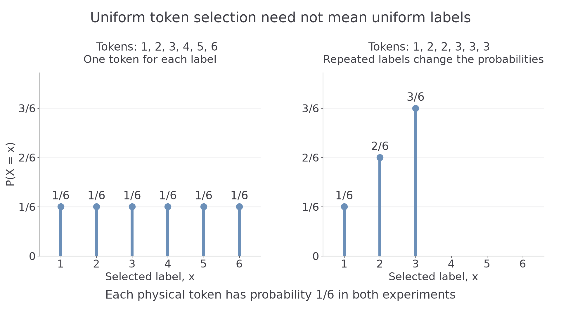
A box contains one token for each integer from 1 to 6. A token is selected uniformly. Why is the mean label 3.5, and would the same model work for tokens labelled 1, 2, 2, 3, 3, 3? The selection rule and the numerical labels both matter.

With one token of each label, each of the six values has probability $1/6$ . “Uniform” describes equal probabilities, not a guarantee of evenly spread results in a short sequence of selections.

Discrete uniform distribution

For a positive integer $n$ , the discrete uniform distribution on $\{1,2,\ldots,n\}$ has

P(X=x)=\begin{cases} 1/n&x\in\{1,2,\ldots,n\}\\ 0&\text{otherwise} \end{cases}

There are exactly n allowed values. For $n=1$ , the value 1 occurs with probability 1.

An event's probability is its number of allowed values divided by n. Count integers satisfying the event, including endpoints only when the inequality allows them. Non-integer values have probability zero.

Worked example 1: counting an inclusive interval

Question. $X$ is discrete uniform on $\{1,2,\ldots,8\}$ . Find $P(3\leq X\leq6)$ .

Plan. List the integers in the interval and multiply their count by $1/8$ .

\{3,4,5,6\}\quad\Rightarrow\quad P(3\leq X\leq6)=\frac48=\frac12

Answer. $1/2$ .

Check. The four excluded integers are $1,2,7,8$ , so the complementary probability is also $4/8$ , giving total 1.

Keep the distribution and interval bounds, but exclude the upper endpoint. A single integer carries a nonzero probability.

Worked example 2: changing one endpoint

Question. For the same distribution, find $P(3\leq X<6)$ .

Plan. Count again with 6 excluded.

\{3,4,5\}\quad\Rightarrow\quad P(3\leq X<6)=\frac38

Answer. $3/8$ .

Check. Subtract the excluded endpoint's mass from the previous answer: $1/2-P(X=6)=4/8-1/8=3/8$ .

The probability changes at the integers and stays constant as a bound moves between adjacent integers.

Watch out

The integers from a to b inclusive number $b-a+1$ , not $b-a$ . This is a discrete count; an interval's length alone is not its probability.

Count the allowed values in a new distribution.

Conditions for a uniform model

The standard model applies when there are n consecutive integer values starting at 1, every one is possible, and each has the same probability. Equal spacing alone does not establish equal probability. A loaded die still has equally spaced labels.

In the opening second box, selecting a physical token uniformly does not select a numerical label uniformly. Label 1 occurs on one token, label 2 on two and label 3 on three. Its complete distribution is

$x$	1	2	3
$P(X=x)$	$1/6$	$2/6$	$3/6$

[DIAGRAM: asset_name: Uniform tokens and non-uniform labels; asset_slug: aqa7367-uniform-labels; caption: Six equally likely tokens give uniform labels only when each label occurs equally often; description: Two probability spike plots share the same scales. Left, tokens labelled 1 through 6 give six masses of 1/6. Right, tokens labelled 1, 2, 2, 3, 3, 3 give masses 1/6 at 1, 2/6 at 2 and 3/6 at 3. All token lists, spike heights and axes are labelled.]
Six equally likely tokens give uniform labels only when each label occurs equally often

More generally, a discrete uniform distribution can be defined on any finite set of distinct values with equal masses. However, the mean and variance formulae for $1,\ldots,n$ require those particular values. A uniform label from $5,6,7,8$ has four possible values, not eight. Write it as $U+4$ , where U is uniform on $1,2,3,4$ , before adapting the formulas. A uniform label from $2,4,6,8$ has four possible values with spacing 2, so it needs a scale change too.

Relabelling one-to-one preserves equal masses: if $Y=c+dU$ with $d\ne0$ , different values of U give different values of Y. For $d<0$ , their order reverses when Y's values are sorted; their probabilities remain attached. If $d=0$ , all labels collapse to the single value c. The calculation of mean and variance for these cases follows in the next part.

Do not confuse a finite discrete uniform model with a continuous uniform, or rectangular, model on an interval. The discrete model assigns positive probability to each of finitely many allowed values. A continuous uniform model permits every real value in its interval and assigns probability zero to any single exact value. It uses interval lengths to calculate probabilities. The two models have different variance formulas.

Key idea

Identify the random quantity being recorded. Equally likely objects give equally likely values only when the numbers of objects producing those values are equal.

Test that condition rather than just looking for equally spaced labels.

Proving the mean and variance

Equal masses let you use the finite sums you already know. For $U$ uniform on $\{1,2,\ldots,n\}$ , each moment is an ordinary sum divided by n. Pairing equally weighted endpoints also suggests the mean: $(1+n)/2$ .

Discrete uniform moments

For positive integer $n$ ,

E(U)=\frac{n+1}{2},\qquad \operatorname{Var}(U)=\frac{n^2-1}{12}

These discrete uniform formulas are not printed in the exam booklet. Learn them and understand the proof. The booklet's arithmetic-series formula on page 4 gives $\sum_{r=1}^n r=n(n+1)/2$ by using endpoints 1 and n. Page 7 supplies $\sum_{r=1}^n r^2=n(n+1)(2n+1)/6$ .

The second moment is the bridge between the two finite sums and the variance.

Continue this lesson.

You’re previewing NovaLearn without an account. Create a free account to read the rest.

Create free account

Last Accessed

Core Pure

Mechanics

Statistics

Discrete Mathematics

SA6, SA7 - The discrete uniform model

Equally likely integers from 1 to n

Conditions for a uniform model

Proving the mean and variance

Continue this lesson.

Learn faster with Nova