SD1 - Mixed distributions | AQA A-Level Further Mathematics

A random quantity can put some probability at an exact value and spread the rest across an interval. You will combine point masses with continuous area, recognise jumps in a cumulative distribution function and handle strict and inclusive boundaries correctly.

Point masses and continuous area

A payment is exactly zero with probability $1/4$ , while the remaining probability is spread uniformly between 0 and 3 pounds. Can its CDF jump even though some payments vary continuously? We need a model that keeps both kinds of probability.

A point mass, also called an atom, is a positive probability attached to one exact value. Here $P(X=0)=1/4$ . On $0<x<3$ , write $g(x)$ for the density of the continuous contribution. Its area must be $3/4$ , because the atom has already used $1/4$ of the total probability.

Mixed distribution

A mixed distribution has both point masses and a continuous contribution with positive total probability. For any event, add the masses of the atoms it contains and the area of its continuous contribution. The function $g$ alone is not a pdf for the whole distribution: its area is less than 1.

If you first choose the continuous branch, its conditional density is $1/3$ on $(0,3)$ . Multiplying by the branch probability $3/4$ gives the unconditional contribution $g(x)=(3/4)(1/3)=1/4$ . This distinction prevents counting the continuous branch twice.

Worked example 1: sharing the total probability

Question. $P(X=0)=1/4$ , and the only remaining probability has constant continuous density $g(x)=k$ on $0<x<3$ . Find $k$ and $P(1<X<2)$ .

Plan. Make atom plus area equal 1, then integrate only over the requested interval.

\frac14+\int_0^3 k\,\mathrm{d}x=1 \quad\Longrightarrow\quad 3k=\frac34 \quad\Longrightarrow\quad k=\frac14.

The event $(1,2)$ contains no atom, so

P(1<X<2)=\int_1^2\frac14\,\mathrm{d}x=\frac14.

Answer. $k=1/4$ , probability $1/4$ .

Check. Three intervals of length 1 each contribute $1/4$ ; with the atom, the total is $3(1/4)+1/4=1$ .

Keep the continuous interval fixed but increase the atom. Less probability is available for continuous payments.

Worked example 2: increasing the atom

Question. Now $P(Y=0)=2/5$ , with remaining constant continuous density $g(y)=k$ on $0<y<3$ . Find $k$ and $P(1<Y<2)$ .

Plan. Subtract the atom from 1 before dividing by the support width.

\frac25+3k=1\quad\Longrightarrow\quad k=\frac15, \qquad P(1<Y<2)=\int_1^2\frac15\,\mathrm{d}y=\frac15.

Answer. $k=1/5$ , probability $1/5$ .

Check. The conditional chance of landing in this middle third, given $Y>0$ , is $1/3$ . Multiplying by $P(Y>0)=3/5$ gives $1/5$ .

Normalisation uses both components, not just the smooth part.

Watch out

Wrong: set $\int g(x)\,\mathrm{d}x=1$ and then add an atom. That gives too much probability. For a mixed model, $\sum p_i+\int g(x)\,\mathrm{d}x=1$ , with all masses and density values nonnegative.

Find the continuous contribution for a fresh mixture.

Jumps in a CDF

A CDF still means $F(x)=P(X\leq x)$ . When the boundary reaches an atom, the entire mass is collected at once, producing a jump. Between atoms, the CDF accumulates continuous area as before.

Write $F(c^-)=\lim_{x\to c^-}F(x)=P(X<c)$ for its value just before $c$ . Then

P(X=c)=F(c)-F(c^-).

The value at a jump is its upper value, because $F(c)$ includes $X=c$ . A CDF is right-continuous: approaching from values just above $c$ recovers $F(c)$ . Changing the value at a jump changes the distribution, unlike changing one isolated density height.

Worked example 3: an atom at the lower boundary

Question. Find the complete CDF when $P(X=0)=1/4$ , with continuous contribution $g(x)=1/4$ on $0<x<3$ , and no other probability.

Plan. Include the atom as soon as the bound reaches zero, then add continuous area.

For $0\leq x<3$ ,

F(x)=\frac14+\int_0^x\frac14\,\mathrm{d}t=\frac14+\frac x4.

Answer.

F(x)=\begin{cases} 0,&x<0,\\ (1+x)/4,&0\leq x<3,\\ 1,&x\geq3. \end{cases}

Check. $F(0^-)=0$ and $F(0)=1/4$ , so the jump is $1/4$ . At 3 the left limit is 1: there is no atom at 3.

Move only the atom from 0 to 3. The continuous contribution stays unchanged, but its accumulated area now comes before the jump.

Worked example 4: an atom at the upper boundary

Question. Find the complete CDF when $P(Y=3)=1/4$ , with $g(y)=1/4$ on $0<y<3$ , and no other probability.

Plan. Accumulate the continuous area up to 3, then add the atom at 3.

F(y)=\int_0^y\frac14\,\mathrm{d}t=\frac y4 \quad(0\leq y<3).

Answer.

F(y)=\begin{cases} 0,&y<0,\\ y/4,&0\leq y<3,\\ 1,&y\geq3. \end{cases}

Check. $F(3^-)=3/4$ and $F(3)=1$ , so $P(Y=3)=1/4$ . Both tails and total probability are correct.

The graph shows why the domain at the jump must be precise.

[DIAGRAM: asset_name: Moving an atom moves the CDF jump; asset_slug: aqa7367-mixed-cdf; caption: The same continuous contribution has a jump at zero or three according to the atom's location; description: Two CDF graphs compare an atom of one quarter at zero with an atom of one quarter at three. Both have slope one quarter between zero and three. Left has an open circle at (0,0), a filled circle at (0,0.25), then rises to (3,1). Right rises from (0,0) to an open circle at (3,0.75), with a filled circle at (3,1). Dashed vertical segments mark jumps but are not part of either graph. Tails are zero and one.]
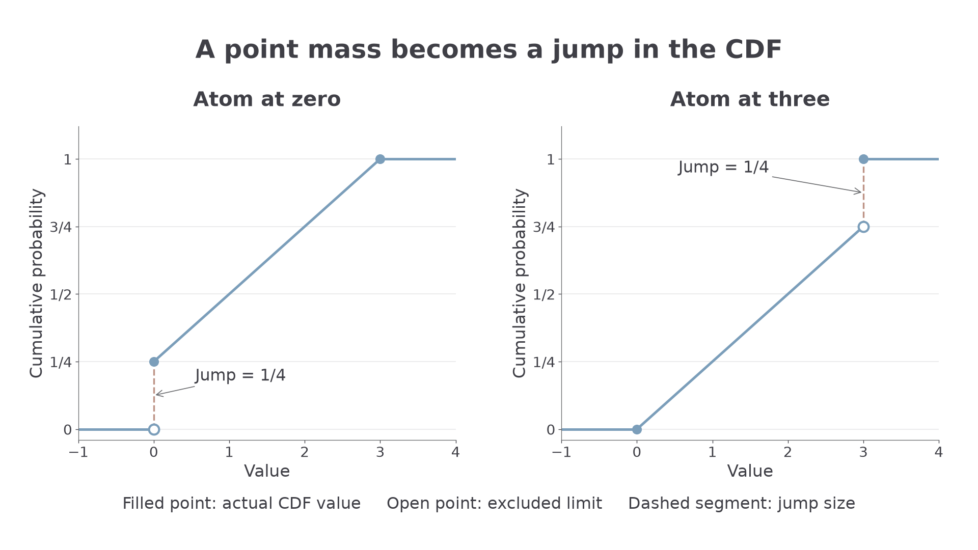
The same continuous contribution has a jump at zero or three according to the atom's location

Differentiating the sloping pieces gives $g=1/4$ for both models. It loses the jump information, so a piecewise derivative alone cannot describe the whole mixed distribution.

Continue this lesson.

You’re previewing NovaLearn without an account. Create a free account to read the rest.

Create free account

Last Accessed

Core Pure

Mechanics

Statistics

Discrete Mathematics

SD1 - Mixed distributions

Point masses and continuous area

Jumps in a CDF

Continue this lesson.

Learn faster with Nova