J1 - Mid-ordinate and Simpson’s rules | AQA A-Level Further Mathematics

Numerical integration estimates a definite integral from a finite set of function values. You will build the mid-ordinate and Simpson’s rules, choose the right points and weights, and judge what a change of step size actually tells you about accuracy.

Build and use the quadrature rules

Can three heights give the exact area under $y=1+x^2$ from $x=0$ to $x=2$ , even though the boundary is curved? Rectangles give one estimate; a curved approximation gives another.

Quadrature means numerical integration. Split $[a,b]$ , with $a<b$ , into $n$ equal subintervals of width $h=(b-a)/n$ . The integral is a signed accumulation: negative heights contribute negatively. Geometric area requires separate treatment of any sign changes.

For the mid-ordinate rule, put one rectangle in each subinterval. Its height is the function value at that subinterval’s midpoint, not its left or right endpoint. Write $x_r=a+rh$ and $y_r=f(x_r)$ , allowing half-integer subscripts for midpoint values. Adding width times height gives the formula.

Mid-ordinate rule

For $n$ equal subintervals, where $n\ge1$ is an integer,

\int_a^b f(x)\,\mathrm{d}x\approx M_n =h\left(y_{1/2}+y_{3/2}+\cdots+y_{n-1/2}\right), \qquad h=\frac{b-a}{n}.

This rule is supplied on page 9 of the examination formula booklet. There are $n$ midpoint heights.

Simpson’s rule instead fits a quadratic through three equally spaced points, covering two subintervals at once. To see its weights, centre those points at $t=-h,0,h$ and write the quadratic as $q(t)=A+Bt+Ct^2$ . Then

\begin{aligned} \int_{-h}^{h}q(t)\,\mathrm{d}t&=2hA+\frac{2h^3C}{3}\\ \frac h3\{q(-h)+4q(0)+q(h)\}&=\frac h3(6A+2Ch^2) =2hA+\frac{2h^3C}{3}. \end{aligned}

The two expressions agree. Adding adjacent pairs counts each shared endpoint twice and gives the composite formula.

Simpson’s rule

For an even number $n\ge2$ of equal subintervals,

\int_a^b f(x)\,\mathrm{d}x\approx S_n =\frac h3\left[y_0+y_n+4(y_1+y_3+\cdots+y_{n-1}) +2(y_2+y_4+\cdots+y_{n-2})\right].

This rule, including the condition that $n$ is even, is supplied on page 9 of the examination formula booklet. For $n=2$ , there are no interior even-indexed terms.

[DIAGRAM: asset_name: Rectangles and a quadratic through the same curve; asset_slug: aqa7367-quadrature; caption: Midpoint rectangles estimate the area; a quadratic fit follows this quadratic exactly; description: Two coordinate panels show y equals one plus x squared from zero to two. The left has two width-one blue rectangles with heights 1.25 and 3.25 at x equals 0.5 and 1.5. The right marks the three Simpson ordinates at zero, one and two, with heights 1, 2 and 5; the quadratic interpolant coincides with the curve. Both panels have the same axes and scale.]
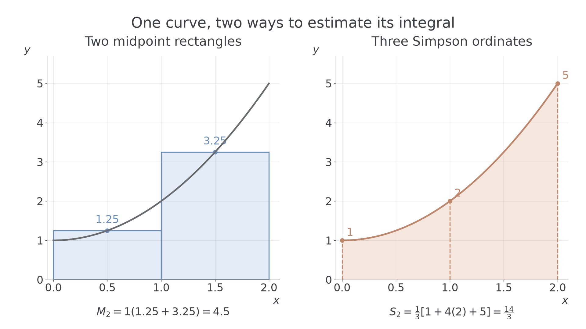
Midpoint rectangles estimate the area

Use both rules on the same integral so that only the shape approximation changes.

Worked example 1: midpoint rectangles

Question. Use two mid-ordinate rectangles to estimate $\int_0^2(1+x^2)\,\mathrm{d}x$ .

Plan. Find the width and the two midpoint heights, then add their rectangle contributions.

\begin{aligned} h&=\frac{2-0}{2}=1 &&\text{two equal subintervals}\\ y_{1/2}&=1+0.5^2=1.25,\quad y_{3/2}=1+1.5^2=3.25\\ M_2&=1(1.25+3.25)=4.5. \end{aligned}

Answer. The estimated integral is $4.5$ .

Check. Direct integration gives $[x+x^3/3]_0^2=14/3\approx4.667$ . The rectangle answer is close but is not exact.

Keep the interval and integrand, and change only the rule. Three endpoint heights now describe a quadratic exactly.

Worked example 2: a quadratic fit

Question. Use Simpson’s rule with three ordinates to estimate the same integral, $\int_0^2(1+x^2)\,\mathrm{d}x$ .

Plan. Three ordinates make two subintervals; apply weights $1,4,1$ .

\begin{aligned} h&=\frac{2}{3-1}=1 &&\text{two gaps between three points}\\ (y_0,y_1,y_2)&=(1,2,5)\\ S_2&=\frac13[1+4(2)+5]=\frac{14}{3}. \end{aligned}

Answer. $14/3$ . Here the estimate equals the exact integral because the integrand is the fitted quadratic.

Check. The antiderivative $x+x^3/3$ again gives $14/3$ , independently of the numerical weights.

This is the opening surprise: a finite set of heights can determine an exact integral for a suitable function. It does not make Simpson’s rule exact for every curved boundary.

Watch out

For two mid-ordinate rectangles on $[0,2]$ , use $x=0.5,1.5$ . For Simpson’s rule with three ordinates, use $x=0,1,2$ . Midpoints and endpoint ordinates belong to different formulas.

Try the same comparison with a changed coefficient.

Use equal widths and the correct sample points

A list of heights alone does not determine an integral: their horizontal spacing matters too.

For mid-ordinate data, locate the subinterval boundaries first. Four equal subintervals on $[1,3]$ have width $0.5$ , boundaries $1,1.5,2,2.5,3$ , and midpoint positions $1.25,1.75,2.25,2.75$ . The midpoints are half a step inside the interval. For Simpson data on the same four subintervals, use all five boundary positions instead.

Equal spacing

A common-width quadrature formula requires every gap between consecutive boundary positions to equal $h$ . For midpoint samples, consecutive sample positions also differ by $h$ , and the two outer boundaries are half a step beyond the first and last midpoints.

For unequal subintervals, you may still add individual midpoint rectangles as $\sum_i \Delta x_i f(m_i)$ , using each actual width and midpoint. The composite Simpson weights with one common $h$ cannot simply be applied to unevenly spaced data. If more values can be calculated from a function, choose a suitable equally spaced grid. A table of measurements does not authorise inventing extra values.

Worked example 3: midpoint data on a known interval

Question. Four equal subintervals cover $[1,3]$ . Their midpoint heights are $2,3,5,6$ , in order. Use the mid-ordinate rule to estimate the integral.

Plan. Obtain the width from the boundaries, then multiply the sum of heights by that width.

\begin{aligned} h&=\frac{3-1}{4}=0.5\\ M_4&=0.5(2+3+5+6)=8. \end{aligned}

Answer. The estimated integral is $8$ .

Check. The mean sampled height is $16/4=4$ . Interval length times mean height is $2\times4=8$ , the same total by a different calculation.

Now stretch the horizontal interval by a factor of two, leaving the four heights unchanged. The integral estimate must stretch by the same factor.

Worked example 4: the same heights over twice the width

Question. Four equal subintervals now cover $[1,5]$ , with midpoint heights $2,3,5,6$ . Estimate the integral by the mid-ordinate rule and state the midpoint positions.

Plan. Recalculate the width; locate each sample half a step from its left boundary.

\begin{aligned} h&=\frac{5-1}{4}=1\\ (m_1,m_2,m_3,m_4)&=(1.5,2.5,3.5,4.5)\\ M_4&=1(2+3+5+6)=16. \end{aligned}

Answer. The estimate is $16$ , using midpoints $1.5,2.5,3.5,4.5$ .

Check. The mean height is still $4$ , but the interval length is now $4$ , giving $4\times4=16$ . Doubling the horizontal scale doubled the estimate.

The same scale factor multiplies Simpson’s estimate because its formula also has a single factor of $h$ .

Watch out

Wrong: four subintervals mean $h=(b-a)/5$ . Correct: divide by four. Five is the number of boundary ordinates, not the number of widths.

Use a fresh interval and fresh midpoint data.

Continue this lesson.

You’re previewing NovaLearn without an account. Create a free account to read the rest.

Create free account

Last Accessed

Core Pure

Mechanics

Statistics

Discrete Mathematics

J1 - Mid-ordinate and Simpson’s rules

Build and use the quadrature rules

Use equal widths and the correct sample points

Continue this lesson.

Learn faster with Nova