SB1–SB3 - The Poisson distribution

Conditions and notation

A sensor detects an average of three particles per minute. Could it detect none in the next minute, and how could we find that probability? An average of three does not mean one particle must arrive every twenty seconds.

Think of a time line with irregularly spaced detections. A Poisson model describes the number of events in a fixed interval when events occur independently, at a constant mean rate, and singly rather than in simultaneous groups. More precisely, in a very short interval the probability of one event is approximately proportional to its length, while the probability of two or more is negligible in comparison. Counts in disjoint intervals are independent. The same model can apply to events along a length or across an area when the corresponding conditions hold.

For the sensor, let $X$ be the number of particles detected in one minute. Under those assumptions, $X\sim\operatorname{Po}(3)$. A count is dimensionless; “per minute” describes the rate used to obtain its parameter. Zero is a possible count even though the mean is positive. A zero rate gives the limiting degenerate model in which the count is always zero, rather than a positive-rate Poisson process.

A detector that needs a long recovery time after each detection breaks independence: one event suppresses another. A door admitting a crowd together breaks the single-event assumption. A queue with a much higher arrival rate at lunchtime than in the afternoon breaks the constant-rate assumption across the whole period. “At random” alone establishes none of these conditions. Nor must events be exceptionally rare over the whole interval: a Poisson mean can be large.

[DIAGRAM: asset_name: Counts in equal intervals; asset_slug: aqa7367-poisson-intervals; caption: A constant mean rate allows different observed counts in equal intervals; description: A time line from zero to three minutes has three equal shaded one-minute intervals containing two, four and three event marks. The labels distinguish observed counts 2, 4 and 3 from the model mean 3 per minute. Event locations are illustrative, not measured data.]

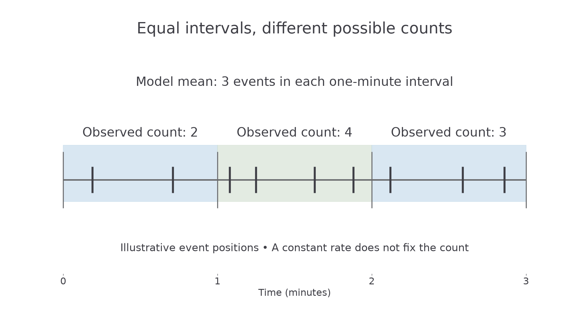
The useful connection is between regularity of the rate and irregularity of individual outcomes. A stable rate does not make successive gaps equal or successive counts equal.

Use the conditions to assess a new model.

Poisson probabilities

To find the chance of no detections, substitute the required count into a probability mass function. A mass function assigns probability to a single integer, just as the finite distributions you already know do.

A calculator's Poisson point-probability function evaluates this formula. Its cumulative function usually gives $F(k)=\operatorname{P}(X\le k)$. Check the event shown on the screen: a cumulative answer is not the probability of exactly $k$. Use a sum, difference or complement for other events:

These hold for integer boundaries with $k\ge0$ and $0\le a\le b$, taking $F(-1)=0$.

Keep the distribution and boundary, but change “exactly two” to “more than two”. This changes one mass into a whole tail.