SD7 - The rectangular distribution
The rectangular distribution models a continuous value spread evenly across a bounded interval. You will find its density and probabilities, decide when equal likelihood is reasonable, and prove its mean, variance and standard deviation.
Uniform density on an interval
If a random length is equally spread between 2 and 8 centimetres, how does its spread change when you add 3 centimetres to every length? First we need to turn “equally spread” into a precise distribution.
For a continuous model, equal likelihood means that intervals of equal length within the support have equal probability. It does not mean a positive equal probability for every individual real number. Each exact value still has probability zero.
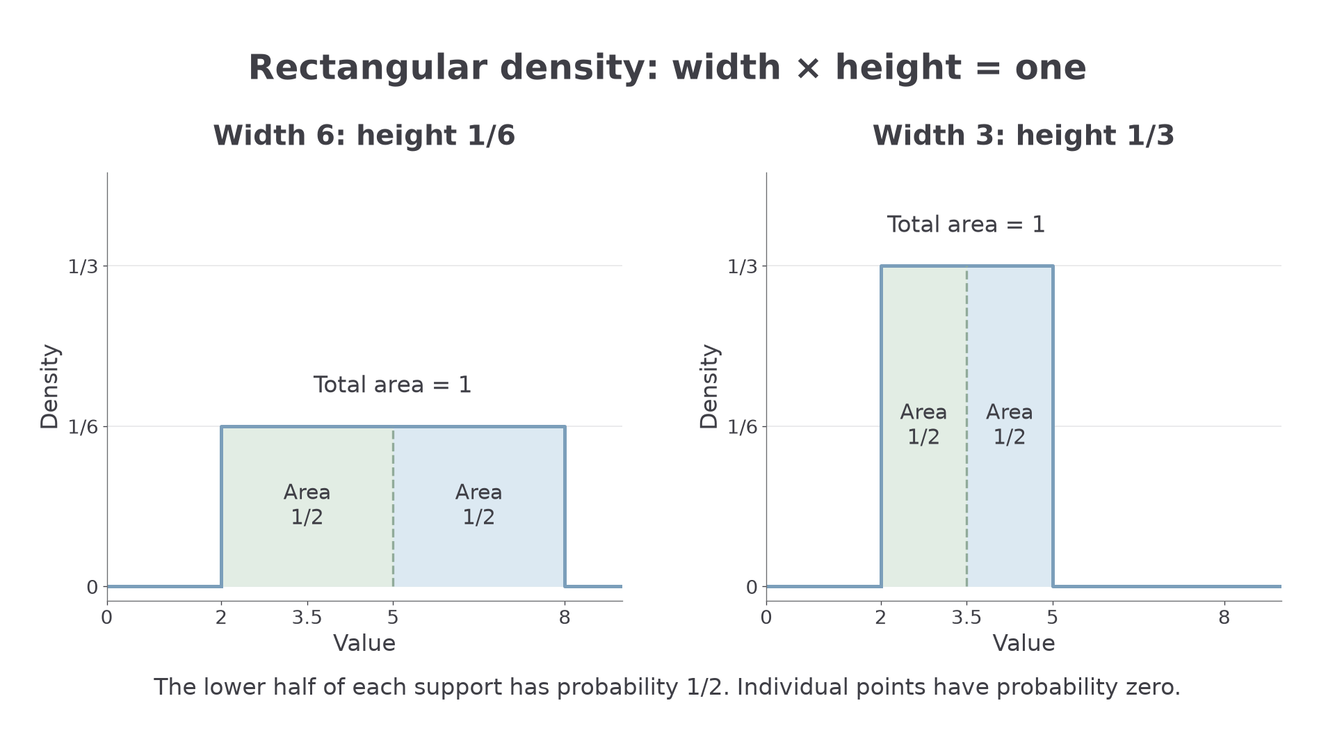
A constant density gives equal areas above equal widths. Between 2 and 8, the rectangle has width 6, so its height must be to give area 1. Each one-centimetre interval then has probability . Generally, if the height is on , normalisation gives . Thus .
Rectangular distribution
For real , a rectangular, or continuous uniform, distribution on has
The density and CDF are not printed in the formula booklet: learn them. Endpoint density values can be allocated differently without changing the distribution.
The CDF is the fraction of the full interval lying to the left of , so it increases along a straight line from 0 to 1.
Worked example 1: a six-unit interval
Question. has a rectangular distribution on . Find its density and .
Plan. Divide total area 1 by the width; then find the area from 2 to 5.
The density is zero elsewhere, and
Answer. Density on , zero otherwise; .
Check. The full rectangle has area , and 5 is the midpoint of its support.
Keep the lower endpoint at 2 and halve the width. The density must double to retain total area 1.
Worked example 2: a narrower interval
Question. has a rectangular distribution on . Find its density and .
Plan. Repeat the width and partial-area calculation for the narrower support.
Answer. Density on , zero otherwise; .
Check. Width 3 times height is 1. Although the height doubles, the probability of the lower half remains .
The density describes probability per unit of the measured variable.
[DIAGRAM: asset_name: Width determines rectangular density height; asset_slug: aqa7367-rectangular-width; caption: Halving the support width doubles the height while total area stays one; description: Two graphs share horizontal and vertical scales. Left shows a rectangle on two to eight with height one sixth. Right shows a rectangle on two to five with height one third. Each rectangle has blue shading and a labelled total area one; the lower half is distinguished in pale sage and labelled probability one half. Zero density outside both supports is shown.]
Watch out
Wrong: use as the height. The height is , using the width, even if is negative. The case is not a rectangular density: its width is zero.
Use a support crossing zero.
Model conditions and probabilities
A rectangular model needs a known finite interval, zero probability outside it, and no preference for one equal-length subinterval over another. These are assumptions about the process; observing a minimum and maximum does not establish uniformity.
For example, suppose a perfectly regular service departs every 10 minutes. If you arrive independently of the timetable and your arrival phase is uniform across a full cycle, your waiting time is rectangular on . “The service runs every 10 minutes” alone is insufficient: people who check the timetable may tend to arrive just before departure. Random arrivals of the service itself would require a different model.
For an interval wholly inside , probability is its width divided by . If the requested interval extends outside the support, intersect it with first. An empty intersection has probability zero.
Worked example 3: an interval within the support
Question. Under the regular-service model above, find .
Plan. Divide the favourable waiting-time width by the full width 10.
Answer. .
Check. The event spans 3 of the 10 minutes; ten disjoint one-minute intervals would each have probability .
Shift the three-minute event to the end of the support. The part beyond 10 contributes no probability.
Continue this lesson.
You’re previewing NovaLearn without an account. Create a free account to read the rest.
Create free account