G2 - Sketching polar curves | AQA A-Level Further Mathematics

A polar graph is traced by changing an angle and travelling the corresponding radius. You will use key values, symmetry and admissible angles to sketch trigonometric curves, then find intersections and tangents at the pole. You will see why setting two radius formulae equal can miss a genuine intersection.

Key angles, symmetry and admissible radii

Can two polar curves meet at the pole without having equal radii at any shared angle there? To recognise that intersection, you first need to know what each curve actually traces.

For $r=2+\cos\theta$ , the point at $\theta=0$ lies 3 units right of the pole. At $\pi/2$ it lies 2 units above it. At $\pi$ , it lies 1 unit left. The radius is a distance from the pole, not a height above the horizontal axis.

Admissible angle

An admissible angle satisfies the stated parameter interval, any domain restrictions in the formula, and the chosen radius convention. In this lesson use $r\geq0$ unless signed radii are explicitly allowed. Thus a value making $f(\theta)<0$ is excluded from $r=f(\theta)$ under this convention.

For $r=2+\cos\theta$ , every angle is admissible because $-1\leq\cos\theta\leq1$ gives $1\leq r\leq3$ . For $r=\sec\theta$ , angles with $\cos\theta=0$ are undefined, and angles with $\cos\theta<0$ give inadmissible negative radii. Do not join across an undefined angle: the curve may escape to infinity.

A sketch needs the locations of the pole, key points and important changes of shape. Make a small table, mark the corresponding rays, then join in increasing angle order. If the shape between two table entries is unclear, add a midpoint rather than guessing. You can use graphing technology to check the tracing, with its radius convention understood.

Symmetry reduces the work. On a domain preserved by the stated change of angle, allowing full-turn adjustments to the same admitted rays:

$f(-\theta)=f(\theta)$ gives reflection in the initial line.
$f(\pi-\theta)=f(\theta)$ gives reflection in the vertical line through the pole.
$f(\theta+\pi)=f(\theta)$ gives a half-turn about the pole.

These are sufficient tests for nonnegative radii; they are not a complete list of every possible symmetry. Periodicity in $r$ alone does not say the point repeats: its ray may have changed.

Worked example 1: a radius that stays positive

Question. Describe a sketch of $r=2+\cos\theta$ , for $0\leq\theta\leq2\pi$ , with $r\geq0$ . Give its symmetry, axis points and whether it meets the pole.

Plan. Bound the radius, use evenness of cosine, then calculate key angles.

1\leq r\leq3,\qquad \cos(-\theta)=\cos\theta

$\theta$	$0$	$\pi/2$	$\pi$	$3\pi/2$	$2\pi$
$r$	$3$	$2$	$1$	$2$	$3$
$(x,y)$	$(3,0)$	$(0,2)$	$(-1,0)$	$(0,-2)$	$(3,0)$

Answer. A closed curve symmetric about the initial line, extending further right than left, with the listed axis points. It does not meet the pole, since $r\geq1$ . As the angle increases, the tracing goes through the upper half first and then the lower half.

Check. At $\theta=2\pi/3$ , $r=3/2$ gives $(-3/4,3\sqrt3/4)$ , between the upper and left axis points. Reflection supplies the corresponding lower point.

Change only the constant term from 2 to 1. That lets the radius reach zero and changes the smooth left-hand boundary into a cusp at the pole.

Worked example 2: a cardioid reaches the pole

Question. Describe a sketch of $r=1+\cos\theta$ , for $0\leq\theta\leq2\pi$ , with $r\geq0$ . Give its symmetry, axis points and pole angle.

Plan. Use the same table and solve $r=0$ separately.

0\leq r\leq2,\qquad 1+\cos\theta=0\ \Longrightarrow\ \theta=\pi

$\theta$	$0$	$\pi/2$	$\pi$	$3\pi/2$	$2\pi$
$r$	$2$	$1$	$0$	$1$	$2$
$(x,y)$	$(2,0)$	$(0,1)$	$(0,0)$	$(0,-1)$	$(2,0)$

Answer. A cardioid, symmetric about the initial line, with a cusp at the pole at $\theta=\pi$ . Its upper arc runs from $(2,0)$ through $(0,1)$ to the cusp; reflection gives the lower arc.

Check. At $\theta=2\pi/3$ , $r=1/2$ gives $x=-1/4$ . Thus part of the curve lies left of the pole even though its left-hand axis point is the pole itself. Joining the axis points with straight segments would miss that bulge.

The diagrams show what the controlled change has done.

[DIAGRAM: asset_name: Positive-radius curve and cardioid; asset_slug: aqa7367-polar-key-values; caption: Reducing the constant makes the radius reach zero and creates a cusp at the pole; description: Equal-scale plots compare r equals two plus cosine theta and r equals one plus cosine theta. Axis points are marked. The first curve has minimum radius one and does not pass through the pole. The second has minimum radius zero, a cusp at the pole and small arcs to its left.]
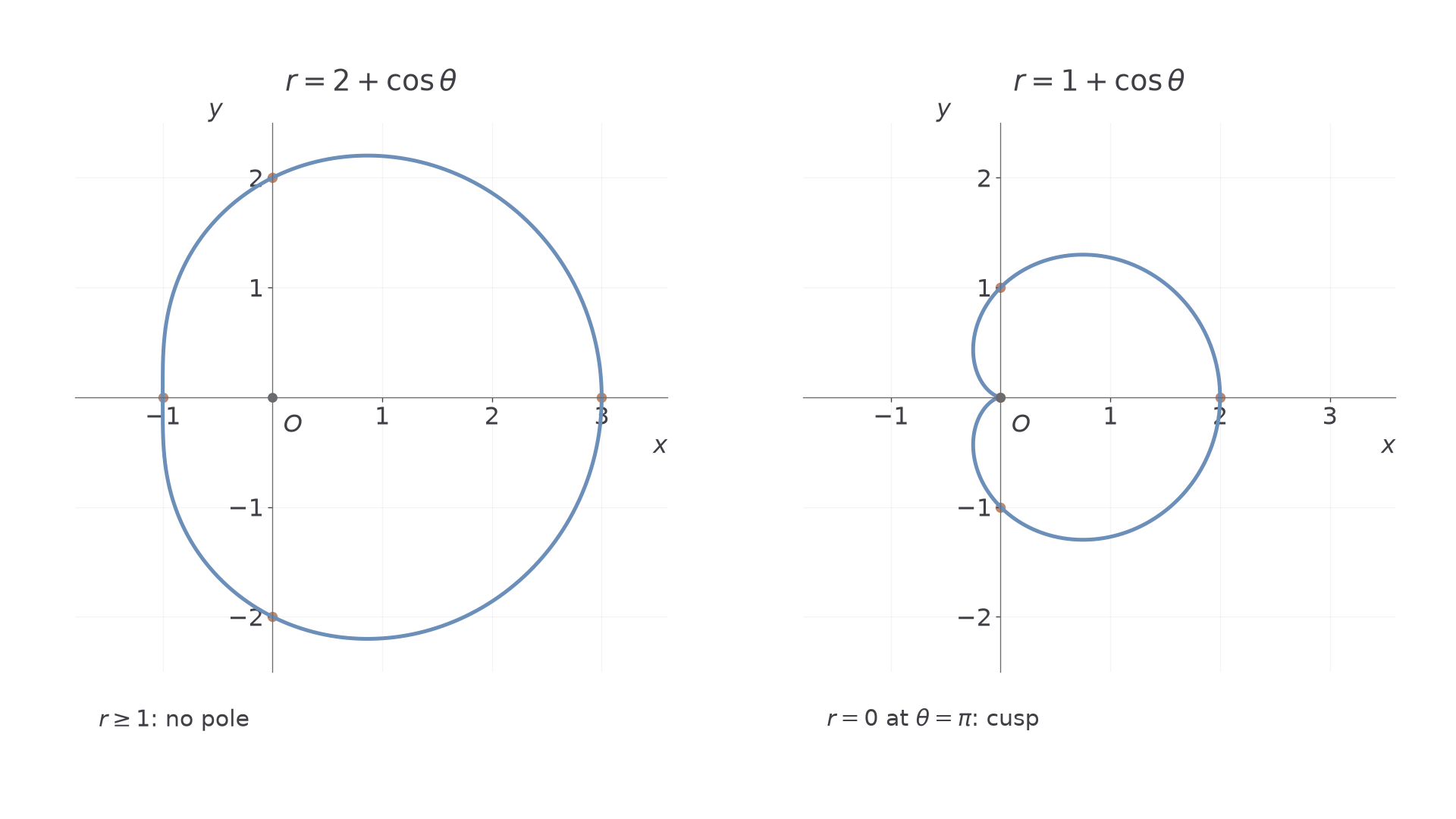
Reducing the constant makes the radius reach zero and creates a cusp at the pole

A smooth sketch should preserve these features rather than look like a join-the-dots polygon.

Watch out

Wrong: “At $\theta=\pi$ , radius 1 means the point $(1,0)$ .” The ray points left, so the point is $(-1,0)$ . Calculate the direction and radius together. Check for zero radius as well as axis crossings.

Repeat the cardioid calculation with a new scale.

Standard trigonometric curves

A familiar trigonometric function does not necessarily give a familiar Cartesian graph. In $r=4\cos\theta$ , cosine supplies a radius on a turning ray. It does not give a vertical coordinate plotted against $\theta$ .

Cartesian conversion identifies the curve exactly:

r=4\cos\theta\ \Longrightarrow\ x^2+y^2=4x \ \Longrightarrow\ (x-2)^2+y^2=4

It is a circle of radius 2 through the pole, centred 2 units along the initial line. With $r\geq0$ , one full tracing uses $-\pi/2\leq\theta\leq\pi/2$ . A change of $\pi$ in angle does not need to mean half a circle: here this entire interval has length $\pi$ , yet traces the whole circle.

Worked example 3: tracing a cosine circle

Question. Give the key points and tracing direction of $r=4\cos\theta$ , for $-\pi/2\leq\theta\leq\pi/2$ and $r\geq0$ .

Plan. Evaluate the endpoints, centre angle and two intermediate angles.

\begin{array}{c|ccccc} \theta&-\pi/2&-\pi/4&0&\pi/4&\pi/2\\ r&0&2\sqrt2&4&2\sqrt2&0\\ (x,y)&(0,0)&(2,-2)&(4,0)&(2,2)&(0,0) \end{array}

Answer. Trace the circle from the pole around its lower half to $(4,0)$ , then around its upper half back to the pole. Its centre is $(2,0)$ and radius 2.

Check. Each listed point satisfies $(x-2)^2+y^2=4$ . The lower half appears first because its angles are negative.

Change only cosine to sine, rotating the locus and its angle interval through $\pi/2$ .

Worked example 4: tracing a sine circle

Question. Give the key points and tracing direction of $r=4\sin\theta$ , for $0\leq\theta\leq\pi$ and $r\geq0$ .

Plan. Use the same stages of the tracing with each angle increased by $\pi/2$ .

\begin{array}{c|ccccc} \theta&0&\pi/4&\pi/2&3\pi/4&\pi\\ r&0&2\sqrt2&4&2\sqrt2&0\\ (x,y)&(0,0)&(2,2)&(0,4)&(-2,2)&(0,0) \end{array}

Answer. A circle with centre $(0,2)$ and radius 2, traced from the pole around the right side to $(0,4)$ , then down the left side to the pole.

Check. The Cartesian equation is $x^2+(y-2)^2=4$ , and rotating Worked example 3's points by a right angle gives exactly these points.

Other common shapes follow the same method. A positive constant radius $r=a$ gives a circle centred at the pole. For $a>0$ , $r=a(1+\cos\theta)$ is the right-facing cardioid from the first part; replacing cosine by sine rotates it upwards. More generally, $r=a+b\cos\theta$ , with $a>b>0$ , stays away from the pole and is symmetric about the initial line. The values of $a$ and $b$ determine its shape; symmetry alone does not determine where the pole sits inside it.

Continue this lesson.

You’re previewing NovaLearn without an account. Create a free account to read the rest.

Create free account

Last Accessed

Core Pure

Mechanics

Statistics

Discrete Mathematics

G2 - Sketching polar curves

Key angles, symmetry and admissible radii

Standard trigonometric curves

Continue this lesson.

Learn faster with Nova