D11 - Modulus and reciprocal graphs
The same graph can generate two very different new graphs by replacing each output with its modulus or its reciprocal. You will sketch these from a given function, tracking fixed levels, zeros, excluded inputs and asymptotes rather than relying on a table of unrelated points.
Sketching modulus and reciprocal graphs
What happens to the point when you replace a function's output by its modulus or reciprocal? The input stays 3. The new output is either or , so the point becomes or . Neither operation swaps the coordinates.
For a point on , the output transformations are
The modulus graph keeps the parts on or above the horizontal axis and reflects the parts below. The reciprocal graph keeps the sign of every nonzero output, but large magnitudes become small and small nonzero magnitudes become large. For example, 4 becomes , while becomes .
Reciprocal graph
The graph of consists of the points for which is defined and nonzero. It is a reciprocal of the output, not an inverse function: and mean different operations.
Start with a few labelled points, then use continuous branches and limiting behaviour to join them. As nonzero outputs on a branch approach zero, their reciprocals become unbounded in magnitude. Where the original outputs become unbounded in magnitude, their reciprocals approach zero.
Worked example 1: two transformations of a line
Question. Sketch the key features of and for .
Plan. Transform useful output values and examine what happens near the original zero .
The modulus graph is a V with vertex , left branch and right branch . Its domain is all real numbers.
For the reciprocal, approaching 1 from the left gives a small negative denominator, so the output tends to ; approaching from the right gives . Far from 1, the denominator grows in magnitude, so the output approaches zero.
Answer. The modulus graph has vertex and vertical-axis intercept . The reciprocal graph has asymptotes and , vertical-axis intercept , a negative left branch and a positive right branch.
Check. The identities and hold on their respective domains. In particular, at , the transformed outputs are 2 and , answering the opening question for this function.
Now multiply the original line's outputs by 2, without moving its zero. This doubles the modulus outputs but halves the reciprocal outputs.
Worked example 2: scaling before taking a reciprocal
Question. Sketch the key features of and for .
Plan. Use the previous graphs and track how doubling each original output changes the new ones.
The modulus graph keeps vertex , with gradients and 2, and passes through . The reciprocal still has asymptotes and , but now passes through and . Its branches keep the same signs.
Answer. A steeper V with unchanged vertex, and a reciprocal curve whose finite outputs are half those in Worked example 1. The reciprocal domain is .
Check. At , , so both transformed outputs equal 1. At , , so the modulus output is 1 while the reciprocal output is . Both match the formulas above.
The first line and its two transformed graphs show the two different operations clearly.
[DIAGRAM: asset_name: One line and its modulus and reciprocal; asset_slug: aqa7367-output-transformations; caption: Modulus reflects negative outputs while reciprocation creates two branches around a missing zero; description: Three coordinate panels show y equals x minus 1, y equals modulus of x minus 1, and y equals 1 divided by x minus 1. Matching points at x equals 0, 2 and 3 are marked. The middle graph is a V with vertex (1,0). The right graph has dashed vertical asymptote x equals 1 and horizontal asymptote y equals 0, with the left branch negative and right branch positive.]
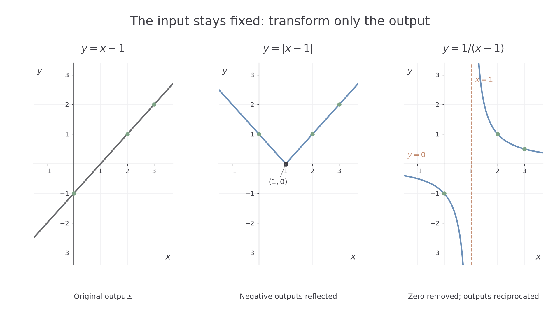
In a sketch, mark asymptotes with dashed lines and let the curve approach them consistently. A branch that first approaches an asymptote and then turns away without a mathematical reason misrepresents its limiting behaviour.
Watch out
Wrong: reciprocal graphs reflect in the line . That describes exchanging input and output when an inverse function exists. A reciprocal keeps fixed and changes to .
Describe the same features for a fresh scaled line.
Zeros, exclusions, asymptotes and fixed levels
The transformed graph inherits information from the original, but different features transform differently. A zero remains a zero under modulus; it is excluded under reciprocation. An input where was undefined stays undefined under both operations.
The fixed levels of reciprocation solve , so and or . Thus points of the original graph on and remain in the same place on its reciprocal. Under modulus, every point at a non-negative level stays in place, while a point at level moves to level 1.
Key idea
A reciprocal graph has no zero: the reciprocal of a finite nonzero real number cannot equal zero. It may approach zero, but a missing original input cannot be filled merely because a simplified formula has a finite value there.
Read limits branch by branch. If approaches a nonzero constant , its reciprocal approaches , which need not be zero. If becomes unbounded near an excluded input, the reciprocal approaches zero there, but that input remains excluded. A hole is an excluded point with a finite limiting output; it is not a vertical asymptote.
Worked example 3: an original asymptote becomes a hole
Question. Let , with . Find the zero and vertical asymptote of . For , find the domain, asymptotes, hole and points fixed by reciprocation.
Plan. Preserve the original domain, exclude the original zero, and then simplify the reciprocal on that domain.
The modulus has zero and vertical asymptote ; reflecting a branch does not bound its magnitude. It also approaches level 1 at both far ends.
For , the original zero becomes the vertical asymptote . The rewritten form shows horizontal asymptote . As approaches 2, the simplified formula approaches 0, but the original is undefined at 2, so has a hole at , not a zero.
To find the fixed points, solve the original level equations:
Answer. For : zero , vertical asymptote . For : domain , asymptotes and , hole , and one fixed point .
Check. , whose reciprocal is . Also and , so their product is 1; neither graph's horizontal asymptote is zero.
Double only the original function's outputs. The zero and original excluded input stay put, while the horizontal limiting level and fixed-point inputs change.
Worked example 4: fixed levels after scaling
Question. Let , with . Find the corresponding features for and .
Plan. Retain the original exclusion and zero, then solve for the fixed points.
The modulus still vanishes at and has vertical asymptote ; its horizontal limiting level is now 2. The reciprocal still excludes and 2, has vertical asymptote , and approaches zero at the hole . Its far-end level is now .
Answer. For : zero , vertical asymptote . For : domain , asymptotes and , hole , and fixed points and .
Check. and , so reciprocation leaves both points fixed. The entire formula also confirms the halved horizontal level and unchanged excluded inputs.
The hole needs an open circle on the reciprocal sketch, even though the simplified curve would otherwise pass smoothly through it.
[DIAGRAM: asset_name: Reciprocation with an inherited hole; asset_slug: aqa7367-reciprocal-hole; caption: The original pole at x equals 2 remains an excluded input after reciprocation; description: Two panels compare f(x) equals (x plus 1) divided by (x minus 2) with its reciprocal (x minus 2) divided by (x plus 1). The original graph has vertical asymptote x equals 2, horizontal asymptote y equals 1 and zero at minus 1. The reciprocal has vertical asymptote x equals minus 1, horizontal asymptote y equals 1, and an open circle at (2,0), explicitly labelled excluded. The common fixed point (one half, minus 1) is marked on both.]
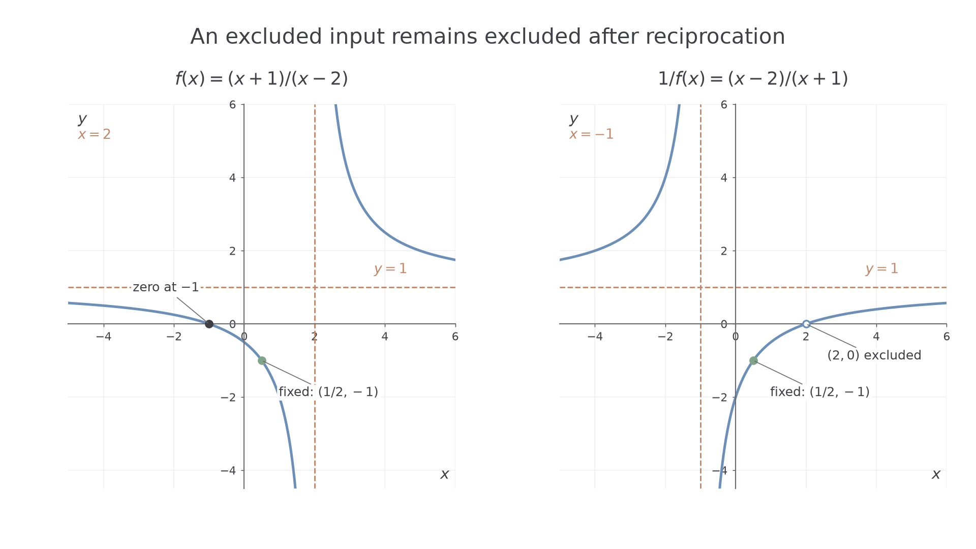
The opening point rule remains reliable even in these more complicated graphs: transform only existing outputs, and never manufacture an output at a missing input.
Watch out
Wrong: every reciprocal graph has horizontal asymptote . That is true when the original magnitude grows without bound at the relevant far end. If the original tends to a nonzero constant , the reciprocal tends to .
Use a new rational function to track these features independently.
Quick Recap
- Modulus changes to , keeping the original domain.
- Reciprocation changes to , excluding zeros as well as missing original inputs.
- The reciprocal fixed levels are 1 and ; use limits to determine asymptotes.
- A reciprocal may approach zero at a hole, but cannot equal zero.
The point stays under modulus and becomes under reciprocation.