SD1, SD2 - Probability density functions
A measurement can take any value in an interval, so a list of separate probabilities is no longer enough. SD1 introduces probability density and its connection to area; SD2 uses that area to calculate interval probabilities. You will also see why a density can exceed 1 even though a probability cannot.
A nonnegative density with total area one
Can a probability graph have a height of 1.6 without breaking the rules of probability? To answer that, we must distinguish the height of a curve from the area beneath it.
Think of a measured time, rather than a count of arrivals. In an ideal continuous model, the time may lie anywhere in a range. A smooth version of a relative-frequency histogram describes how probability is spread across that range: narrow intervals near a high part of the curve receive more probability than equally narrow intervals near a low part.
Probability density function
A probability density function, or pdf, , describes a continuous random variable by area. It must satisfy
The support specifies where values can occur. Give the density there and set it to zero elsewhere. The support can contain more than one interval.
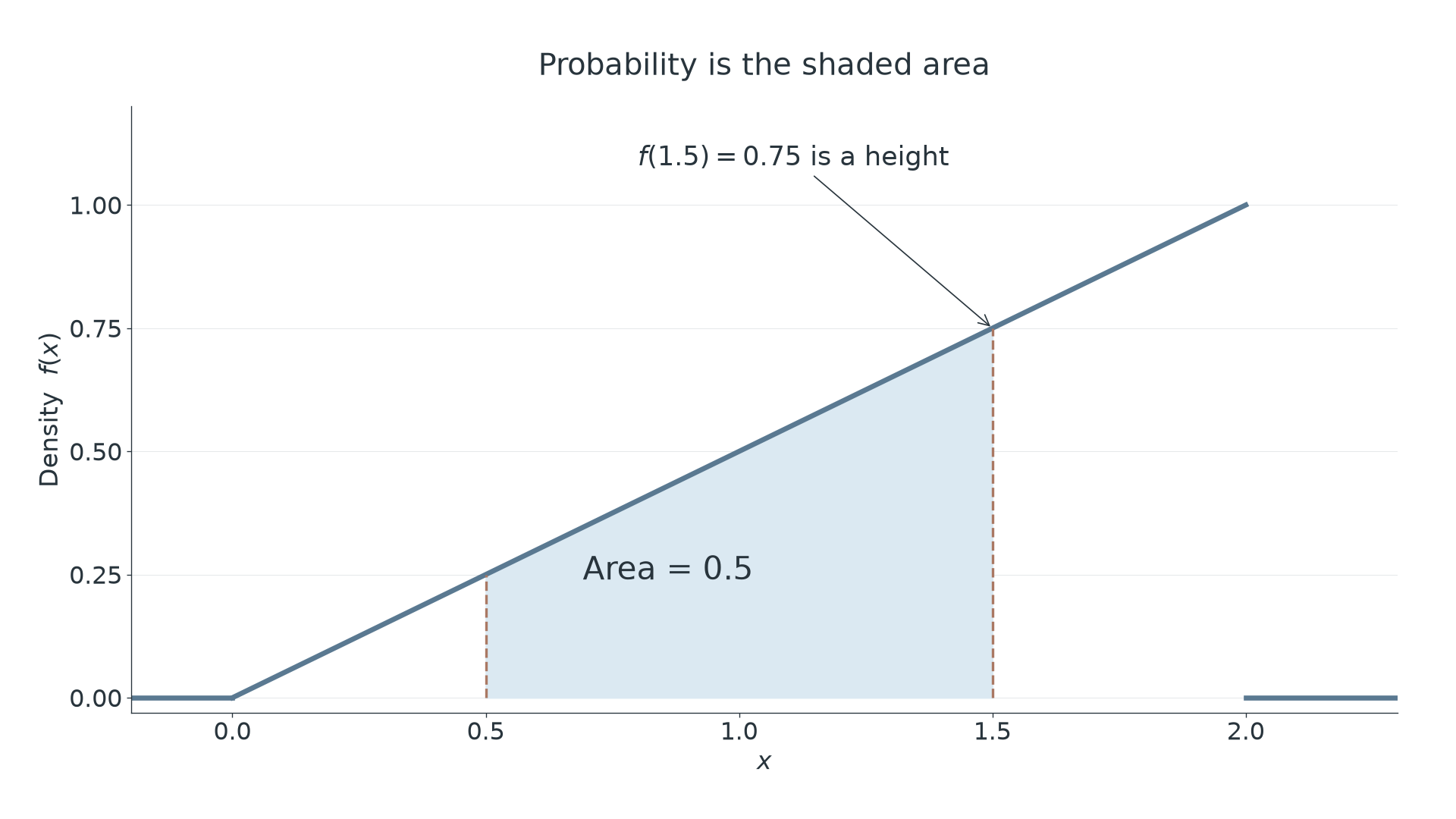
For example, on , and zero otherwise, is nonnegative and has triangular area . The rising height means that equal-width intervals towards 2 have larger probability. It does not attach probability to the exact number .
If the formula contains an unknown constant, the area condition determines it. The sign condition must still be checked.
Worked example 1: normalising a rising density
Question. A density is for , and zero otherwise. Find .
Plan. Integrate over the stated support, equate the result to 1, then check nonnegativity.
Why use limits 0 and 2? They describe the entire region carrying probability; the density is zero outside it.
Answer. . Then throughout the support.
Check. The resulting straight-line graph is a triangle with base 2 and height 1, so its area is 1 independently of the integration.
Keep the same support and reverse the slope. This changes where the probability is concentrated, while preserving the triangular shape.
Worked example 2: normalising a falling density
Question. A density is for , and zero otherwise. Find .
Plan. Normalise over the same interval, now integrating the falling expression.
Thus . Since on , this gives a valid density.
Answer. , with probability now concentrated towards the lower end.
Check. Reflection in the vertical line turns the first triangle into this one. Reflection preserves area, so the same constant makes sense.
Area alone is insufficient. The function on , zero elsewhere, has integral 1, but is negative for . Negative area would give a negative interval probability, so it is not a pdf.
Watch out
Wrong: “The integral is 1, so it is a density.” Check both requirements: total area 1 and nonnegative density throughout the stated support.
Apply both requirements to a new interval.
Interval probabilities are integrals
An interval probability is the area under the density over that interval. Integration adds the small strips of area together.
For a short interval of width near a point where the density is continuous, its probability is approximately . Adding these products and taking a limit explains the integral rule.
Probability from density
For a variable described by a pdf and ,
Use the relevant piece of on each part of the interval; outside the support the contribution is zero. This density rule is required knowledge and is not printed in the AQA formula booklet.
The height tells you how densely probability is packed; height multiplied by width gives area. The graph shows this for the density from Worked example 1.
[DIAGRAM: asset_name: Probability is shaded area; asset_slug: aqa7367-density-area; caption: Under f(x) equals x over 2 on zero to two, the area from 0.5 to 1.5 is one half; description: A coordinate graph shows the rising line f(x) equals x over 2 from (0,0) to (2,1), with zero density outside the interval. Pale blue shading under the line between x equals 0.5 and x equals 1.5 is labelled probability equals 0.5. Dashed verticals mark both bounds. A note distinguishes the height f(1.5) equals 0.75 from the shaded probability.]
Continue this lesson.
You’re previewing NovaLearn without an account. Create a free account to read the rest.
Create free account