J2 - Euler’s method | AQA A-Level Further Mathematics

A differential equation tells you a curve’s gradient even when you do not have its equation. Euler’s method uses those gradients to build an approximate solution from an initial value. You will organise the updates, work backwards from a given estimate, and compare step sizes without confusing numerical precision with model accuracy.

Follow a tangent from an initial value

A curve passes through $(0,1)$ and satisfies $\mathrm{d}y/\mathrm{d}x=x+y$ . How can you estimate its height at $x=0.2$ without first solving the equation? At the starting point its gradient is $0+1=1$ . Moving $0.1$ horizontally along that tangent changes the height by $0.1\times1$ .

A first-order differential equation of the form $\mathrm{d}y/\mathrm{d}x=f(x,y)$ supplies the gradient at a point. An initial value $y(x_0)=y_0$ selects a starting point. In Euler’s method, you follow the tangent for a short horizontal step, then use the new approximate point to obtain the next gradient. The line segments approximate the solution curve; they are not usually pieces of the exact curve.

[DIAGRAM: asset_name: Two tangent steps from an initial value; asset_slug: aqa7367-euler-tangents; caption: Euler follows the current tangent, then recalculates the gradient at the approximate point; description: A coordinate graph shows the exact solution y equals 2 e to the x minus x minus one, from x equals zero to 0.25, and a blue Euler polygon through (0,1), (0.1,1.1) and (0.2,1.22). Dashed vertical guides mark x equals 0.1 and 0.2. The first segment is labelled slope 1; the second slope 1.2. The exact curve is separately labelled for comparison.]
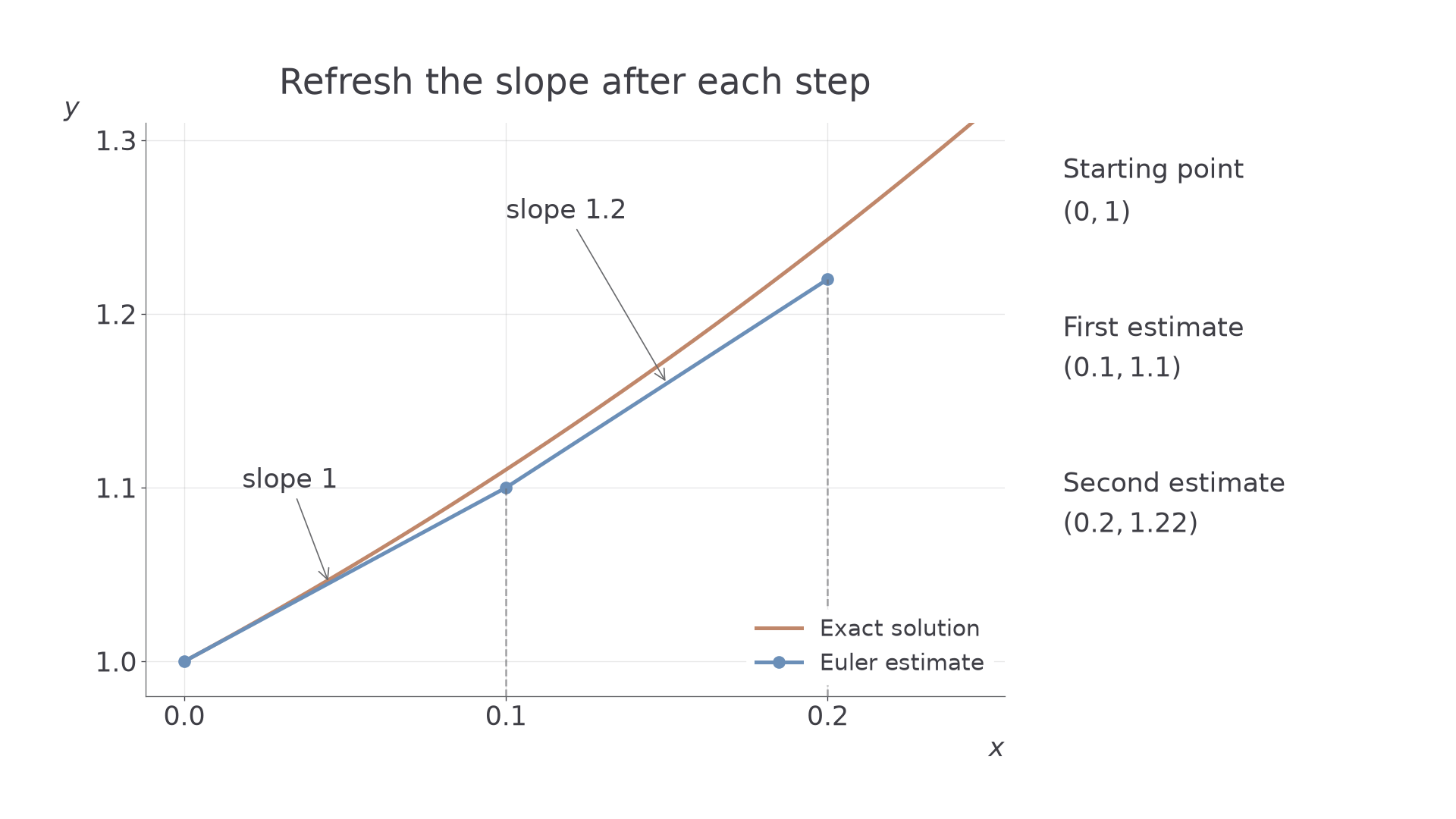
Euler follows the current tangent, then recalculates the gradient at the approximate point

The tangent at $(x_r,y_r)$ has equation $y-y_r=f(x_r,y_r)(x-x_r)$ . Put $x=x_r+h$ to get the update.

Euler’s method

For $\mathrm{d}y/\mathrm{d}x=f(x,y)$ ,

x_{r+1}=x_r+h,\qquad y_{r+1}=y_r+h f(x_r,y_r).

This recurrence is supplied on page 9 of the examination formula booklet. Use a nonzero step small enough to resolve the solution’s changes and evaluate $f$ only where it is defined. A positive $h$ steps right; a negative $h$ steps left.

The required number of equal steps from $x_0$ to $b$ is $N=(b-x_0)/h$ . Choose $h$ so that $N$ is a nonnegative integer when equal steps are required. Do not label an estimate at a nearby grid point as the value at $b$ .

Worked example 1: two forward steps

Question. For $\mathrm{d}y/\mathrm{d}x=x+y$ , $y(0)=1$ , use Euler’s method with $h=0.1$ to estimate $y(0.2)$ .

Plan. Take two steps; each gradient uses the current point before either coordinate is changed.

\begin{aligned} f(0,1)&=1, & y_1&=1+0.1(1)=1.1, &x_1&=0.1\\ f(0.1,1.1)&=1.2, & y_2&=1.1+0.1(1.2)=1.22, &x_2&=0.2. \end{aligned}

Answer. $y(0.2)\approx1.22$ .

Check. The exact function $y=2e^x-x-1$ satisfies both $y'=x+y$ and $y(0)=1$ . It gives $y(0.2)\approx1.242806$ , so the numerical estimate is plausible but not exact.

Keep the equation and starting point, changing only the direction of travel. A negative step reverses the horizontal move; it does not change the differential equation.

Worked example 2: two backward steps

Question. For the same initial-value problem, use $h=-0.1$ to estimate $y(-0.2)$ .

Plan. Take two leftward tangent steps, retaining the signed value of $h$ .

\begin{aligned} f(0,1)&=1, & y_1&=1-0.1(1)=0.9, &x_1&=-0.1\\ f(-0.1,0.9)&=0.8, &y_2&=0.9-0.1(0.8)=0.82, &x_2&=-0.2. \end{aligned}

Answer. $y(-0.2)\approx0.82$ .

Check. The verified exact function gives $2e^{-0.2}+0.2-1\approx0.837462$ . The positive initial slope is consistent with a decrease in height when stepping left.

When $f$ depends only on $x$ , the rule reduces to $y_{r+1}=y_r+h f(x_r)$ . For positive steps, summing the changes gives a left-endpoint rectangle approximation to the integral of the derivative. Euler’s method therefore connects tangent geometry with numerical integration.

Watch out

Wrong: $y_1=1+0.1f(0.1,1)$ . A forward Euler step from $(0,1)$ uses the gradient at $(0,1)$ , not at the destination’s horizontal coordinate.

Practise stepping left with a fresh initial value.

Keep the update order consistent

The two coordinates in a gradient must come from the same row of the calculation.

A safe table has columns $r,x_r,y_r,f(x_r,y_r)$ . First evaluate the gradient from that row. Then calculate both next coordinates from the stored row. Using the new $x$ with the old $y$ changes the algorithm, as does using an already updated height in the old gradient.

Do not round the height after every row unless the question requests it. Store extra digits and round the requested estimate at the end. The table’s displayed height can have fewer digits than the stored value, provided the subsequent calculation retains the latter.

Worked example 3: a gradient containing a quotient

Question. For $\mathrm{d}y/\mathrm{d}x=x/y$ , $y(1)=2$ , use $h=0.2$ to estimate $y(1.4)$ .

Plan. Take two steps and form each quotient from one complete row; the denominator must be nonzero.

$r$	$x_r$	$y_r$	$x_r/y_r$
0	$1$	$2$	$0.5$
1	$1.2$	$2.1$	$4/7$
2	$1.4$	$31/14$	not needed

\begin{aligned} y_1&=2+0.2\frac12=2.1\\ y_2&=2.1+0.2\frac{1.2}{2.1}=\frac{31}{14}\approx2.214286. \end{aligned}

Answer. $y(1.4)\approx2.214286$ .

Check. Separating variables gives $y^2=x^2+3$ on the positive branch selected by $y(1)=2$ . It gives $y(1.4)=\sqrt{4.96}\approx2.227106$ , close to the estimate. Every numerical denominator was positive.

The same stored-row rule lets you infer an unknown starting height. Keep the quotient equation and step size; change the starting height from a given value to an unknown.

Continue this lesson.

You’re previewing NovaLearn without an account. Create a free account to read the rest.

Create free account

Last Accessed

Core Pure

Mechanics

Statistics

Discrete Mathematics

J2 - Euler’s method

Follow a tangent from an initial value

Keep the update order consistent

Continue this lesson.

Learn faster with Nova