SF1, SF2, SF4 - Exponential distributions

Conditions for an exponential model

A detector records particles at a constant mean rate, independently and singly. If no particle has appeared for a minute, is one now “due”? A long empty spell need not make the next event more imminent.

In a homogeneous Poisson process, events occur at a constant positive mean rate, counts in disjoint intervals are independent, and events occur singly. More precisely, for a very short interval of length $h$, the probability of one event is approximately $\lambda h$, and the probability of two or more is negligible compared with $h$. These are the process conditions behind the Poisson count model.

A Poisson variable counts how many events occur in a fixed interval. An exponential variable measures the nonnegative waiting time to the next event in this process. Here $\lambda>0$ is a rate per unit time, not a mean count in an arbitrary interval. Counts over a duration $t$ have Poisson mean $\lambda t$.

This is a model assumption, not a consequence of the word “random”. A component whose failure tendency increases as it wears out does not have a constant failure rate. A detector with a recovery period after each event prevents immediate new detections, breaking the process conditions. Rush-hour arrivals across a whole day have a varying rate. Equally spaced departures produce a different waiting model even if a traveller arrives unpredictably.

In a lifetime setting, a constant failure rate means the chance of failing in a short additional period, conditional on having survived so far, does not depend on age. It does not mean the density of the total lifetime is constant. Exponential lifetimes are concentrated towards shorter durations, as the next part shows.

Identify the appropriate random quantity.

The density and cumulative distribution

For a rate $1/2$ per minute, the exponential density starts at height $1/2$ and decays as time increases. This makes a short wait more likely than an equally wide interval much later. It leaves some probability beyond every finite time.

The density is nonnegative. Its total area is

because $\lambda>0$. Accumulating only as far as $t\geq0$ gives $F(t)=1-\mathrm{e}^{-\lambda t}$. Differentiating that CDF returns the density for $t>0$.

Double only the rate. The same two-minute interval now captures more of the probability.

The density and CDF express the same distribution on different vertical scales.

[DIAGRAM: asset_name: Exponential densities and cumulative probabilities; asset_slug: aqa7367-exponential-curves; caption: Increasing the rate concentrates waiting times nearer zero and makes cumulative probability rise faster; description: Two side-by-side plots show rate one half in blue and rate one in sage for nonnegative time. The left plot shows densities one half times exp minus t over two and exp minus t. The right shows their CDFs one minus exp minus t over two and one minus exp minus t, starting at zero and approaching one. A dashed vertical at time two marks CDF values approximately 0.632 and 0.865. The horizontal asymptote one is marked only on the CDF plot.]

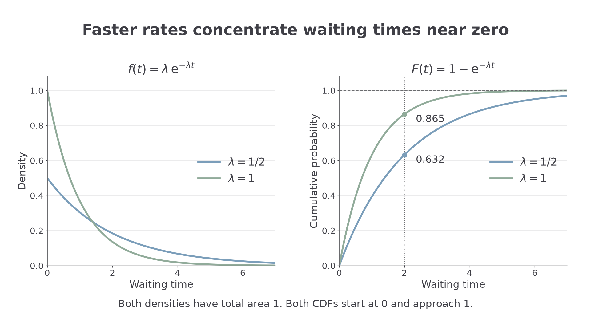
Since this is a pure density, $P(T=0)=0$, even though the density can be positive there. The CDF has $F(0)=0$, no jump at 0, and limit 1 as $t\to\infty$. A zero rate would make the alleged density zero everywhere, so $\lambda=0$ is excluded.

Use both representations for a fresh rate.

Interval and tail probabilities

The survival probability is the chance that the waiting time exceeds a chosen duration. Complementing the CDF makes it particularly simple.

For a negative bound, use the support: $P(T\leq b)=0$ and $P(T>b)=1$ when $b<0$. For an interval crossing zero, integrate from zero. Do not extend the positive-time tail formula to negative times.

Keep the lower boundary, but cap the wait at 5 minutes. Subtract the tail beyond 5 from the tail beyond 3.