SA1, SA2 - Discrete probability distributions

Tables and probability functions

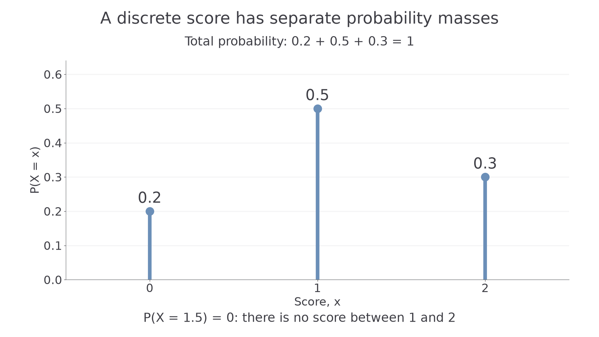
A game awards 0, 1 or 2 points with probabilities 0.2, 0.5 and 0.3. Given that you score at least 1 point, what is the probability you score 2? We first need to distinguish the score from its probability.

A random variable assigns a number to each outcome of a chance experiment. Let $X$ be the score before playing; $x$ denotes a particular possible score. A discrete random variable has a finite or countably infinite set of possible values, rather than every value in an interval. Discrete values need not be integers: a payment could take only the values $0$, $0.50$ and $1.25$ pounds.

For the game, the complete distribution is:

[DIAGRAM: asset_name: Separate probabilities for a discrete score; asset_slug: aqa7367-discrete-score; caption: Probability is attached to each separate score; no intermediate score is possible; description: Three vertical probability spikes at scores 0, 1 and 2 have labelled heights 0.2, 0.5 and 0.3. The horizontal axis is score x and the vertical axis is P(X=x). A note says total probability 0.2 plus 0.5 plus 0.3 equals 1 and P(X=1.5)=0.]

These probabilities describe a model, not the exact frequencies in a short run. If observed values $x_1,x_2,\ldots$ occur with frequencies $f_1,f_2,\ldots$, those $f_i$ are counts. The relative frequencies $f_i/\sum f_i$ can estimate probabilities $p_i$, but they are not automatically the model's exact probabilities.

You already know notation such as $X\sim\mathrm{B}(n,p)$: the symbol $\sim$ means “has the distribution”. Here $\mathrm{B}(n,p)$ is binomial, $n$ is the fixed number of trials, $p$ is the common success probability and $q=1-p$ is the failure probability, with independent binary trials. The game table itself does not assert a binomial model. Later, $E(X)$ will denote its expectation and $\operatorname{Var}(X)$ its variance.

Change only the representation: a function can contain exactly the same information as a table.

Read the support before substituting into any algebraic rule.

Try an algebraic function with a different support.

Valid probability masses

The possible values are mutually exclusive: one observation of $X$ cannot equal two different values at once. Their probabilities therefore add. If the list is exhaustive, one of them must occur, giving total probability 1.

The values themselves may be negative; only their probabilities must be nonnegative. A zero probability is allowed in a table, although that value then lies outside the positive-probability support.