SD6 - Cumulative distribution functions
A cumulative distribution function records all the probability collected up to a chosen value. SD6 connects it to the density through integration and differentiation. You will build complete piecewise functions, handle tails and gaps, and subtract cumulative probabilities to find intervals.
From density to CDF and back
If a density has a gap, does its cumulative probability drop back to zero inside that gap? Imagine moving a vertical boundary from left to right: the area already collected stays collected.
Start with for , zero elsewhere. By the time the boundary reaches , the collected area is
The integration variable is because will be used for the moving upper bound. Replacing 0.5 by produces a function of that bound.
Cumulative distribution function
The cumulative distribution function, or CDF, is
For a variable described by a pdf,
It measures accumulated probability, not density height.
Integration accumulates area; differentiation measures how quickly that area grows.
The density–CDF connection
Where the density is continuous, the fundamental theorem of calculus gives
More generally, a piecewise continuous pdf is recovered by differentiating each smooth piece of its CDF. At a join, may not exist; choose density values at isolated joins without changing probabilities. These pdf/CDF formulae are required knowledge and are not printed in the AQA formula booklet.
The full function must also describe values below and above the support.
Worked example 1: integrating a density
Question. Find the complete CDF when for , and zero otherwise.
Plan. Work below, within and above the support separately.
For , no probability has been collected, so . For ,
For , all the area has been collected, so .
Answer.
Check. , , and the middle piece increases between them. Its derivative is , recovering the supplied density in the interior.
Now reverse the direction for exactly the same distribution. This exposes an important difference between the upper tail of a CDF and the upper tail of a pdf.
Worked example 2: differentiating a CDF
Question. A continuous variable has
Find a pdf.
Plan. Differentiate on the open intervals, then supply harmless endpoint values.
For , . For and , the CDF is constant, so its derivative is zero. At , the left derivative is 3 and the right derivative is 0: there is no two-sided derivative there.
Answer. One valid choice is
Choosing instead would describe the same distribution.
Check. The proposed density is nonnegative and . Reintegrating gives the original CDF, including its value at 1.
A continuous CDF need not have a continuous derivative. The value is fixed by probability, while the density's value at the single point 1 does not affect any area.
Watch out
Wrong: differentiate the middle formula and leave the CDF's upper-tail value 1 in your pdf. A constant differentiates to zero; write the density's zero regions too.
Build a complete function for a shifted support.
Tails, endpoints and gaps
A CDF cannot forget probability as its boundary moves right. It is nondecreasing, lies between 0 and 1, and approaches 0 and 1 in its lower and upper tails respectively.
For a pdf with bounded support, those tails are exactly constant outside the support. For unbounded support, 0 or 1 may be approached without being reached at a finite value. Because a pure pdf assigns no probability to a point, its CDF has no jumps: it is continuous, including at piecewise joins. However, a gap with zero density produces a flat interval.
[DIAGRAM: asset_name: A gap gives a flat cumulative function; asset_slug: aqa7367-cdf-gap; caption: Two density regions of area one half give a CDF that stays at one half across the gap; description: Left shows f(x) equals x on zero to one, x minus two on two to three, and zero otherwise. Each rising triangular region has area 0.5. Right shows F(x) equals x squared over two on zero to one, stays flat at 0.5 on one to two, then rises as 0.5 plus (x minus two) squared over two to reach one at three. Lower and upper tails are zero and one, and all joins are continuous.]
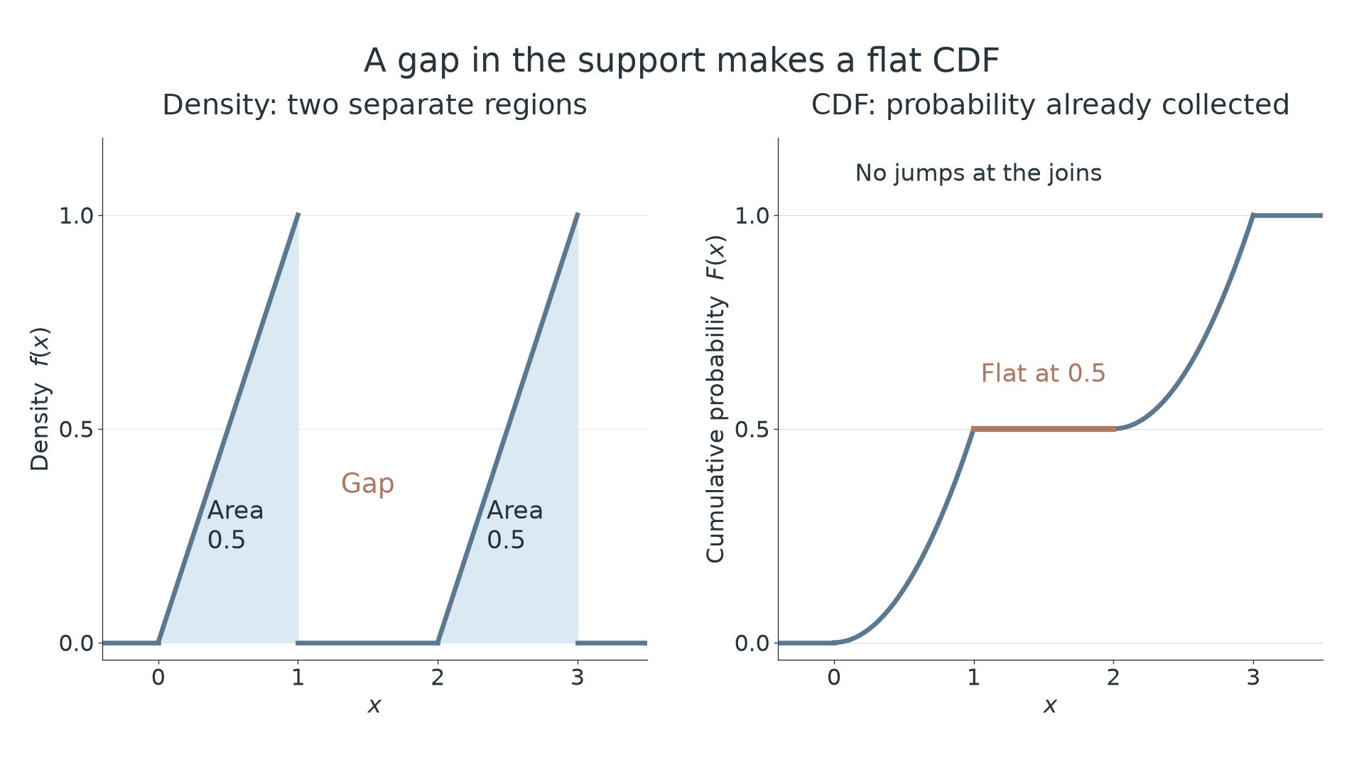
The two triangles in this picture each contribute . In the second region, the CDF must include the first triangle's area as well as the new area.
Continue this lesson.
You’re previewing NovaLearn without an account. Create a free account to read the rest.
Create free account