SE1–SE3 - Chi-squared tests for association | AQA A-Level Further Mathematics

Learn to organise categorical observations, calculate the counts predicted by independence and use a chi-squared test to investigate association. You will check the expected-count condition and combine categories when that is meaningful.

Constructing contingency tables

If two groups choose different travel methods, is that evidence of association or just sampling variation? First, put every observation in the correct cell.

A survey records each person's home area and main travel method. These are two categorical variables: each observation belongs to one category of each variable. One person contributes to one cell, not several. Categories within a variable must be mutually exclusive and cover the observations included in the investigation.

Contingency table

An $n\times m$ contingency table cross-classifies observations using $n$ row categories and $m$ column categories. Its cells contain observed frequencies, $O$ . Marginal totals are the row and column totals; the grand total $N$ is the number of observations. Totals are not extra categories.

Worked example 1: recovering missing cells

Question. Of 100 people, 40 live centrally and 60 live outside the centre. Of the central residents, 24 use public transport. In total, 50 use public transport. Everyone uses either public or private transport. Construct the table.

Plan. Use the stated intersection, then subtract from row and column totals.

\begin{aligned} O_{\text{central, private}}&=40-24=16\\ O_{\text{outer, public}}&=50-24=26\\ O_{\text{outer, private}}&=60-26=34 \end{aligned}

Answer.

Area	Public	Private	Total
Central	24	16	40
Outer	26	34	60
Total	50	50	100

Check. The private column gives $16+34=50=100-50$ ; the two independent ways of obtaining that total agree.

Keep the two area totals and public total fixed, but change the central public count. Other cells must change with it.

Worked example 2: fixed totals constrain the cells

Question. Repeat the construction with 30 central residents using public transport; all totals remain as above.

Plan. Subtract from the same margins, rather than changing only one cell.

40-30=10,\qquad 50-30=20,\qquad 60-20=40

Answer. The rows (Public, Private) are Central $(30,10)$ and Outer $(20,40)$ .

Check. Both columns still total 50, and the rows still total 40 and 60. Changing one count forced changes in three others.

This is association between categories. Recall that $r$ denotes a sample product moment correlation coefficient and $\rho$ its population counterpart. Those describe linear correlation between paired numerical variables. Coding “Central” as 1 and “Outer” as 2 does not turn this investigation into a Pearson correlation test.

Watch out

A $2\times2$ table has four observed cells. Counting the totals as a third row and third column incorrectly calls it $3\times3$ .

Expected counts under independence

If area and transport are independent, the population proportion using public transport is the same in each area. We estimate that common proportion from the whole sample, then apply it to each row total.

In Worked example 1, half the sample uses public transport. Independence therefore predicts half of the 40 central residents, or 20. It predicts half of the 60 outer residents, or 30. An expected frequency is a model prediction; it need not be an integer.

Expected cell frequency

Under the null hypothesis of independence,

E_{ij}=\frac{R_iC_j}{N}

where $R_i$ is the row total, $C_j$ the column total and $N$ the grand total.

Not in the formula booklet: learn it.

Worked example 3: equal column totals

Question. Find expected counts when row totals are 40 and 60 and column totals are 50 and 50, with $N=100$ .

Plan. Multiply each row total by each column proportion.

\begin{aligned} E_{11}=E_{12}&=40\times\frac{50}{100}=20\\ E_{21}=E_{22}&=60\times\frac{50}{100}=30 \end{aligned}

Answer. Expected rows are $(20,20)$ and $(30,30)$ .

Check. Their row totals are 40 and 60 and their column totals are 50 and 50, matching the observed margins.

Change only the column totals to 35 and 65. The row totals stay fixed, but the predicted proportions change.

Worked example 4: unequal column proportions

Question. Find expected counts for row totals 40 and 60, column totals 35 and 65 and $N=100$ .

Plan. Apply proportions 0.35 and 0.65 to each row.

\begin{aligned} (E_{11},E_{12})&=(40\times0.35,40\times0.65)=(14,26)\\ (E_{21},E_{22})&=(60\times0.35,60\times0.65)=(21,39) \end{aligned}

Answer. Expected rows are $(14,26)$ and $(21,39)$ .

Check. The public proportions are $14/40=21/60=0.35$ , exactly the equality independence predicts. If a margin were 36 instead of 35, values such as 14.4 would be legitimate expected counts.

The observed margins are used to fit the independence model. Two different observed tables with the same margins consequently have the same expected table.

Watch out

Wrong: divide by the number of cells. Correct: divide $R_iC_j$ by the grand total $N$ . Keep unrounded expected values for later calculations.

Measuring departure from independence

Simply adding $O-E$ would hide association: the positive and negative departures cancel. Squaring stops that cancellation. Dividing by $E$ measures a departure relative to the scale of the expected count.

Chi-squared statistic

For independent observations in a contingency table, when the expected-count condition is satisfied, under independence

X^2=\sum_{\text{all cells}}\frac{(O-E)^2}{E}

is approximately chi-squared distributed. A large statistic indicates greater disagreement with independence. Each summand is a cell contribution.

The statistic and its approximate chi-squared distribution are in the formula booklet. Its conditions must still be checked.

Use a $2\times3$ table here. The separate lesson on interpretation explains the continuity correction for $2\times2$ tables.

Worked example 5: adding six contributions

Question. An observed table has rows $(30,20,10)$ and $(10,20,30)$ . Its expected counts are all 20. Calculate $X^2$ .

Plan. Calculate one contribution per cell, including zero contributions.

\begin{aligned} X^2&=\frac{10^2}{20}+\frac{0^2}{20}+\frac{(-10)^2}{20} +\frac{(-10)^2}{20}+\frac{0^2}{20}+\frac{10^2}{20}\\ &=5+0+5+5+0+5=20 \end{aligned}

Answer. $X^2=20$ .

Check. There are four departures of magnitude 10, each contributing 5, so $4\times5=20$ .

Halve each departure from 20 while retaining the margins. The statistic falls by a factor of four, because departures are squared.

Worked example 6: halving the discrepancies

Question. The observed rows are now $(25,20,15)$ and $(15,20,25)$ , again with expected counts all 20. Find $X^2$ .

Plan. Replace each nonzero discrepancy of 10 by 5.

X^2=4\times\frac{5^2}{20}=5

Answer. $X^2=5$ .

Check. Relative to Worked example 5, the squared departure multiplier is $(5/10)^2=1/4$ , so $20/4=5$ .

Watch out

Wrong: $(30-20)^2/30$ . The denominator is the model's expected count: $(30-20)^2/20=5$ . Every cell is included, not only the largest departure.

Degrees of freedom and the test decision

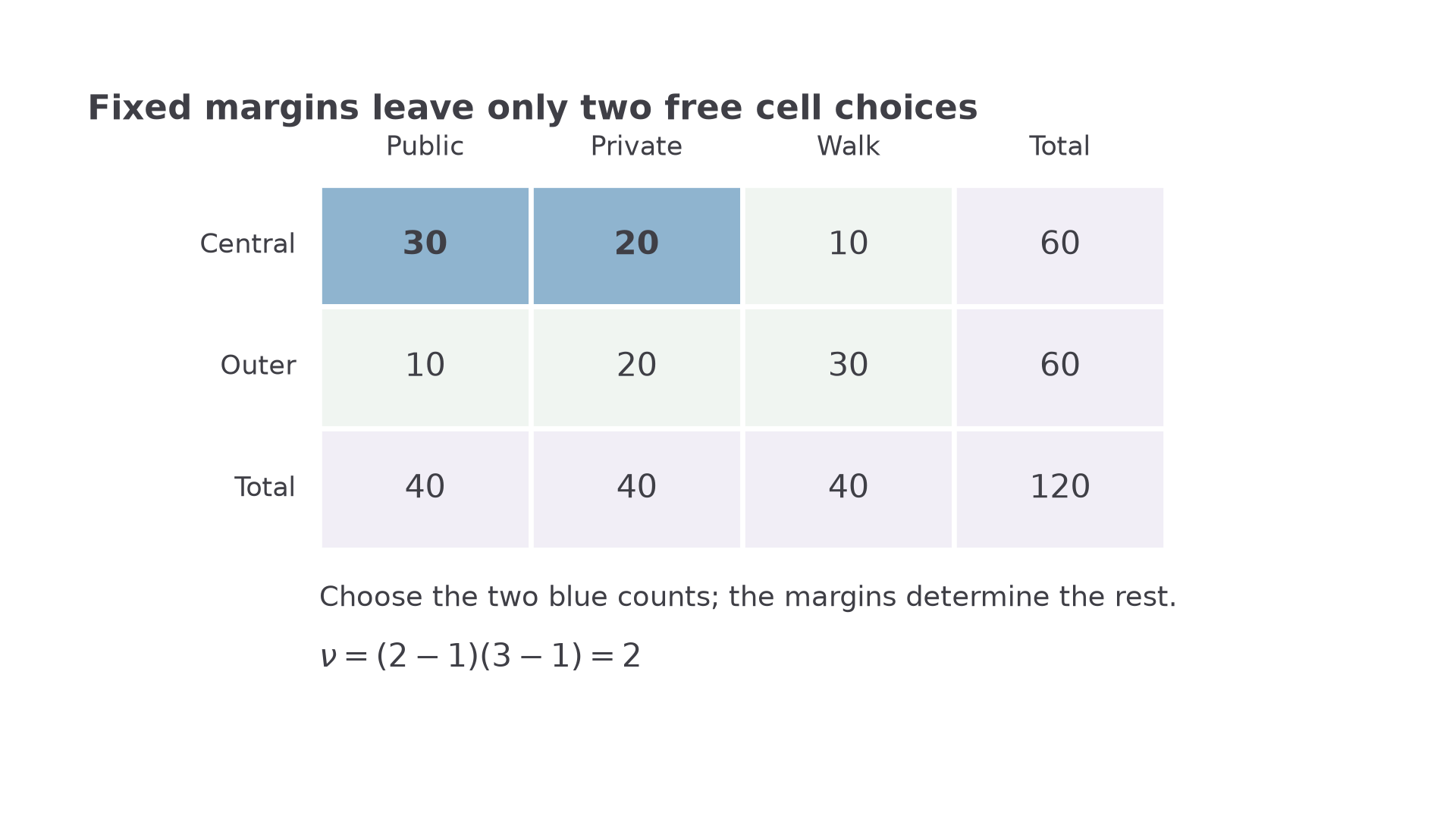
With row and column totals fixed, not every cell can vary independently. In a $2\times3$ table, choosing the first two cells of the first row forces its third cell, then all cells of the second row. Only two choices were free.

[DIAGRAM: asset_name: Free cells in a contingency table; asset_slug: aqa7367-contingency-df; caption: A two-by-three table with fixed margins has two free cell choices; description: A table has rows Central 30 20 10 total 60 and Outer 10 20 30 total 60, with columns Public Private Walk and totals 40 40 40 grand total 120. The first two Central cells are blue. Once these two counts and all margins are fixed, every remaining cell is determined. The degrees of freedom are (2 minus 1) times (3 minus 1), equal to 2.]
A two-by-three table with fixed margins has two free cell choices

Continue this lesson.

You’re previewing NovaLearn without an account. Create a free account to read the rest.

Create free account

Last Accessed

Core Pure

Mechanics

Statistics

Discrete Mathematics

SE1–SE3 - Chi-squared tests for association

Constructing contingency tables

Expected counts under independence

Measuring departure from independence

Degrees of freedom and the test decision

Continue this lesson.

Learn faster with Nova