DD2 - Graphical optimisation
For two decision variables, the constraints become a picture of all permitted choices. You will locate an optimum using vertices and parallel objective lines, recognise when an optimum is absent or shared, and check whole-number decisions carefully. The geometry explains why trying every possible point is unnecessary.
Feasible regions and objective lines
If two products earn £3 and £4 per unit, can making four of the first and two of the second beat six of the first? When products share resources, maximising either quantity alone can miss a better combination; the profit weights decide which direction is valuable.
You already know that a linear inequality describes one side of a straight line. Draw its boundary using equality and test a point away from the boundary to choose the correct side. A solid boundary is included for or . Intersect every permitted half-plane, including nonnegative or minimum-quantity constraints.
Feasible region and vertices
The feasible region consists of points satisfying every constraint. A vertex is a corner of this region. A point on an included boundary is feasible if it also meets all the other constraints; a crossing of two boundary lines outside the region is not a feasible vertex.
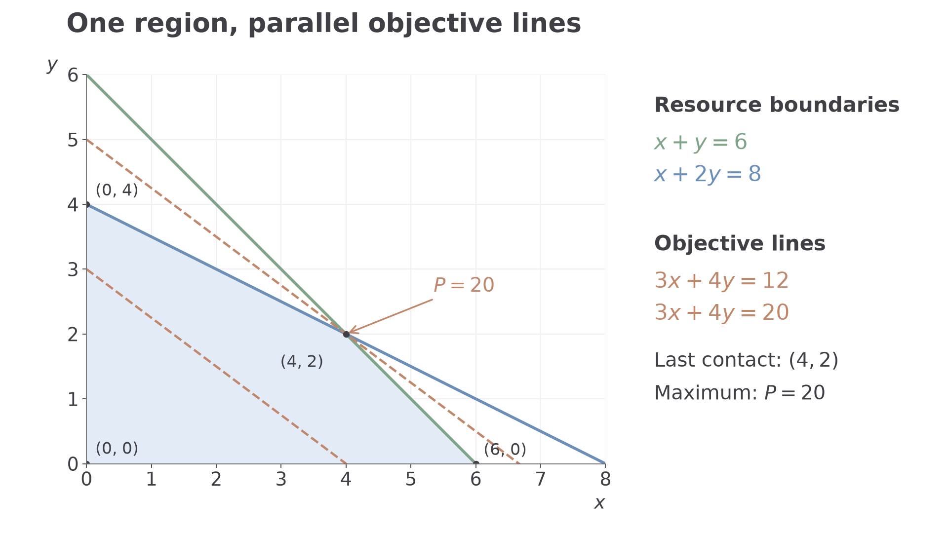
A line joins plans with the same objective value . Varying slides a family of parallel objective lines. The direction of increasing comes from the equation, not from the visual idea of “uphill”: , for example, increases towards larger and smaller .
For a nonempty, closed, bounded polygonal feasible region, a linear objective attains its maximum and minimum. At least one vertex attains each; an entire edge may do so too. Along a segment between vertices the objective is a weighted average of the endpoint values, so an interior point cannot beat both endpoints. This explains the vertex method.
[DIAGRAM: asset_name: A feasible polygon and parallel profit lines; asset_slug: aqa7367-lp-feasible; caption: The last objective line touching the polygon meets the vertex at four comma two; description: A coordinate graph shows x plus y at most six and x plus two y at most eight in the first quadrant. The feasible polygon has vertices (0,0), (6,0), (4,2) and (0,4). Parallel dashed objective lines 3x plus 4y equals 12 and 20 show increasing objective value towards the upper right. The point (4,2) is labelled P equals 20.]
Worked example 1: the best combination
Question. Maximise subject to , , .
Plan. Find the feasible vertices exactly and compare their objective values.
The sloping boundaries meet where subtraction gives , hence . On the axes, both constraints allow at most or . Thus
Answer. The maximum is at . The objective line is the last parallel line to touch the region in the increasing direction.
Check. Adding twice to gives . The proposed point meets both with equality, independently certifying the bound.
Keep the feasible region but reduce the reward for . This changes the slope of the objective lines and can change the best corner.
Worked example 2: changing the objective
Question. Maximise under the same constraints as Worked example 1.
Plan. Reuse the feasible vertices, but calculate the new objective at each.
Answer. The maximum is at . Its objective lines have gradient , rather than , so their last contact is now on the vertical axis.
Check. From , twice the left side is at most 16. Since , . At equality is achieved. The plan making less really does earn more under the new rewards.
The objective belongs to the chosen model: the same permitted plans can have different best answers.
Watch out
Do not assess every boundary intersection automatically. First check it satisfies all inequalities. Keep exact coordinates when comparing close objective values.
Use fresh constraints to practise the full comparison.
Minimum, shared and unbounded optima
Minimisation uses the same objective lines, moved towards decreasing values. Before searching, check whether there are any feasible points and whether the objective can improve without limit.
An infeasible model has an empty feasible region, for example together with . It has no optimum. An unbounded feasible region extends indefinitely, but its objective need not be unbounded. For instance, permits arbitrarily large coordinates, yet has a minimum of zero.
Shared and unbounded objective values
If an objective line coincides with a feasible boundary segment at the optimum, every point on that segment is optimal. An objective is unbounded above if feasible values can exceed every proposed bound, and unbounded below if they can fall below every proposed lower bound. “Unbounded above” means there is no finite maximum, rather than an achievable answer called infinity.
For closed linear-constraint regions, a finite optimum is attained when the region is nonempty. A region may have no vertices, such as a whole half-plane, so do not apply a polygon's vertex list mechanically to every conceivable model. Here the nonnegative constraints keep the examples within the familiar first quadrant.
Worked example 3: a whole edge minimises cost
Question. Minimise subject to , , , .
Plan. Use the direct lower bound on the objective, then find which points on its boundary are feasible.
The third constraint gives . On , write . The other constraints become
Answer. The minimum is , at every point with , including and .
Check. A middle point gives constraint values , so it is feasible and attains 5. No point can do better because . The region extends upwards, but the minimum is finite.
Continue this lesson.
You’re previewing NovaLearn without an account. Create a free account to read the rest.
Create free account