4.5.6.1.4 - Distance-Time Graphs
Distance-time graphs show how the distance travelled by an object changes with time. For this specification point, the key skill is to treat the graph as data: read values from the axes, calculate speed from gradients, and, for Higher tier, use a tangent to find the speed of an accelerating object at one moment.
What the graph shows
On a distance-time graph:
- time is on the horizontal axis
- distance travelled is on the vertical axis
- each point gives the distance travelled at that time
- a straight sloping line means constant speed
- a horizontal line means the object is stationary
- a steeper line means a greater speed
[DIAGRAM: asset_name: Distance-Time Graphs - diagram 1; asset_slug: 069_4_5_6_1_4_distance_time_graphs_diagram1; file: diagram_assets/069_4_5_6_1_4_distance_time_graphs_diagram1.png; recommended_method: deterministic_drawn; description: Exact distance-time graph for a journey with three straight sections. The object travels from 0 m to 20 m in 10 s, stays at 20 m from 10 s to 25 s, then travels from 20 m to 80 m from 25 s to 40 s. Axes are time in seconds and distance in metres. Labels identify constant speed, stationary, faster constant speed, and steeper line means faster speed. Deterministic rendering is required because the axes, coordinates, slopes and section labels are exact assessed graph information.]
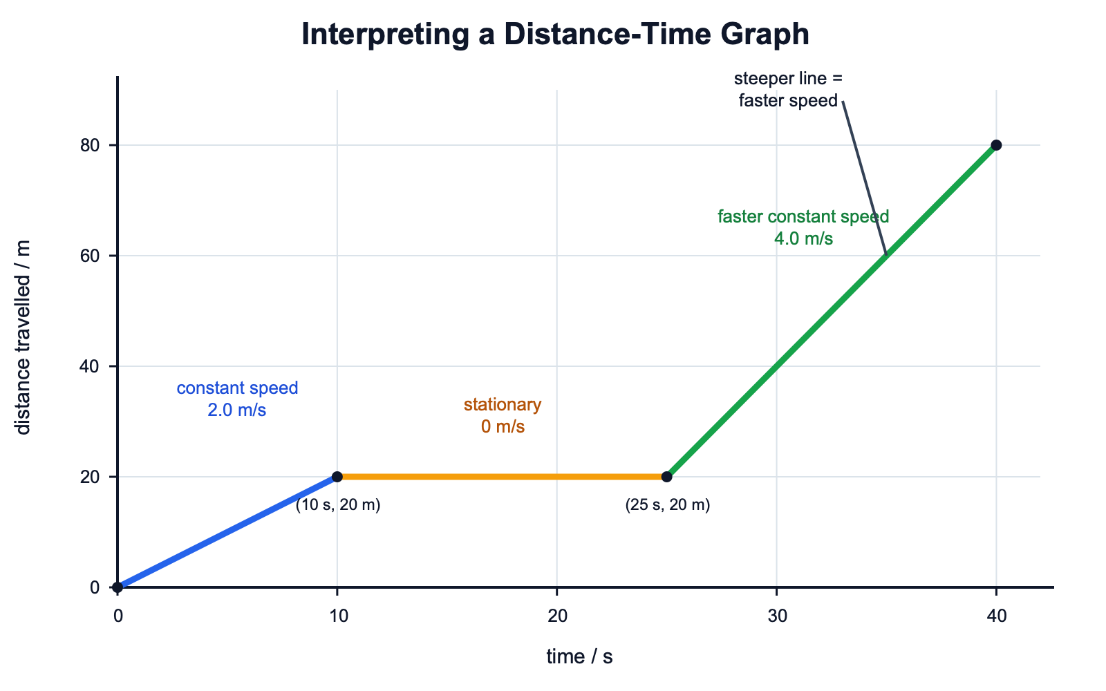
The graph is a compact description of the journey. From 0 s to 10 s, the distance travelled increases by 20 m, so the object is moving. From 10 s to 25 s, the distance stays at 20 m, so the object is stationary. From 25 s to 40 s, the line is steeper, so the object has a greater speed than in the first section.
The graph line is not the path taken by the object. It is a record of distance against time.
Gradient and speed
The speed of an object can be calculated from the gradient of its distance-time graph.
Speed from a Distance-Time Graph
For a straight-line section, choose two points on the line that are easy to read and far apart. Then calculate:
gradient = vertical change / horizontal change
gradient = change in distance / change in time
[DIAGRAM: asset_name: Distance-Time Graphs - diagram 2; asset_slug: 069_4_5_6_1_4_distance_time_graphs_diagram2; file: diagram_assets/069_4_5_6_1_4_distance_time_graphs_diagram2.png; recommended_method: deterministic_drawn; description: Exact distance-time graph showing a straight line through points A at 10 s, 40 m and B at 40 s, 160 m. A gradient triangle is drawn with change in time = 30 s and change in distance = 120 m. The diagram states speed = gradient = 120 m / 30 s = 4.0 m/s. Deterministic rendering is required because the graph values and gradient calculation are exact assessed information.]
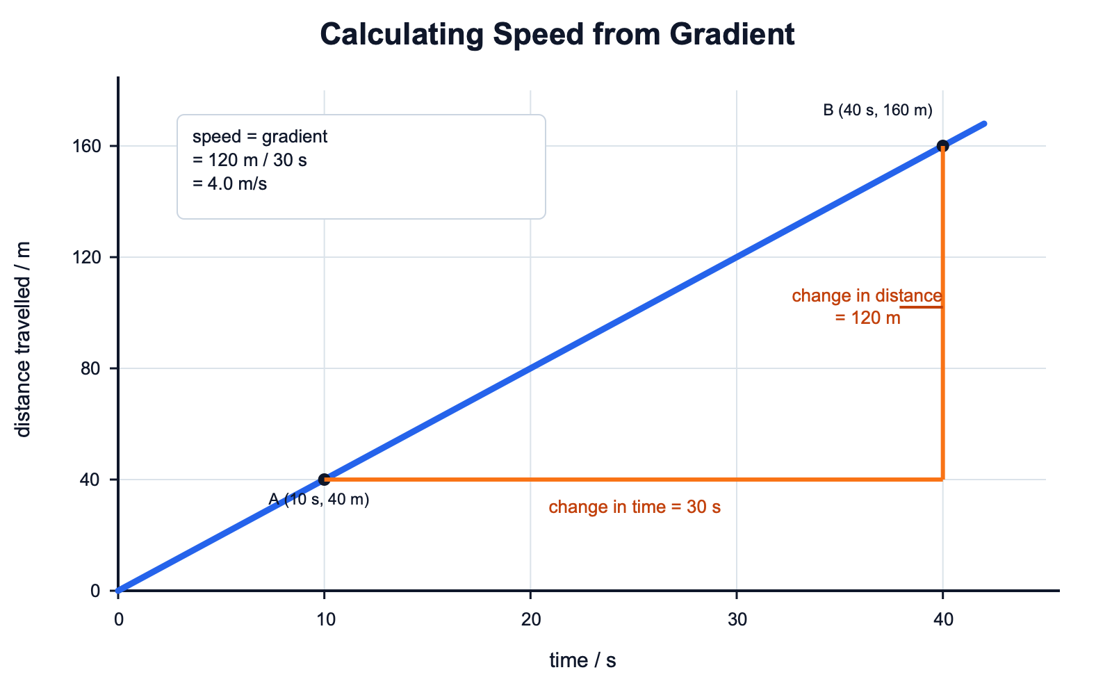
In the diagram:
change in distance = 160 - 40 = 120 m
change in time = 40 - 10 = 30 s
speed = 120 / 30 = 4.0 m/s
The unit comes from the calculation. Distance is in metres and time is in seconds, so the speed is in metres per second, m/s.
For the first and final sections of diagram 1:
| Section | Change in distance | Change in time | Speed |
|---|---|---|---|
0 s to 10 s | 20 m | 10 s | 2.0 m/s |
10 s to 25 s | 0 m | 15 s | 0 m/s |
25 s to 40 s | 60 m | 15 s | 4.0 m/s |
This is why the last section is the fastest: it has the greatest gradient.
Drawing from measurements
Distance-time graphs can be drawn from measurements of distance and time. Use this order:
Continue this lesson.
You’re previewing NovaLearn without an account. Create a free account to read the rest.
Create free account