A.1.6, A.1.10, A.1.11 - Variation, standard deviation and uncertainty
Biological measurements vary, so one average rarely tells the whole story. A.1.6 explains mean, median and mode; A.1.10 adds range and standard deviation to describe spread. A.1.11 shows how to report measurement uncertainty and follow it through a calculation, so that a difference between numbers is not mistaken for stronger evidence than it provides.
Summarising the centre
A summary should describe the measurements that were actually collected, with their units and a sensible precision.
Five seedlings have root lengths of 8, 9, 10, 10 and 13 mm, each recorded to the nearest millimetre. These are five different seedlings, not five readings of one root.
Mean, median and mode
The arithmetic mean is the sum of all values divided by the number of values. The median is the middle value after sorting; for an even number of values, it is the mean of the two middle values. The mode is the most frequent value.
The lengths are already sorted. Their sum is , so the mean is . The third of five values is the median, . The mode is also , because it occurs twice. A mean need not equal an observed value: lengths 8, 9, 10 and 14 mm have unrounded mean , but median . The two middle values, rather than their positions, are averaged. This four-value set has no single most frequent value; report no unique mode rather than choosing one arbitrarily. Other sets can have two modes tied at the greatest frequency.
The mean uses every magnitude, so it is pulled towards an unusually large value. If 13 mm in the five-seedling set is replaced by 23 mm, the mean becomes , while the median and mode remain 10 mm. The median can therefore be a useful description of a typical organism in a skewed sample. It does not make the extreme value unimportant. A genuine exceptionally long root may itself be biologically interesting.
Keep unrounded intermediate values. A calculated mean may reasonably have one more decimal place than individual rounded readings, but additional calculator digits do not show that the measurements were more accurate. Choose final precision from the measurements, uncertainty and task, rather than reporting every displayed digit.
Organising frequencies
A frequency summary shows how many observations fall at each value or in each interval, making the shape of a larger dataset easier to inspect.
For the five root lengths 8, 9, 10, 10 and 13 mm, an exact frequency table is:
| Root length / mm | Frequency |
|---|---|
| 8 | 1 |
| 9 | 1 |
| 10 | 2 |
| 13 | 1 |
| Total | 5 |
Count every observation once. A repeated value contributes repeatedly to the mean: , where is frequency and is the corresponding length. Dividing by four distinct lengths instead of five seedlings would answer the wrong question.
For continuous measurements, group values into non-overlapping class intervals. For a separate complete sample of 6, 8, 9, 10 and 12 mm, choose intervals as follows. The symbol includes a boundary and excludes it, so 8 mm enters the second interval only.
| Root length / mm | Frequency |
|---|---|
| 1 | |
| 2 | |
| 1 | |
| 1 |
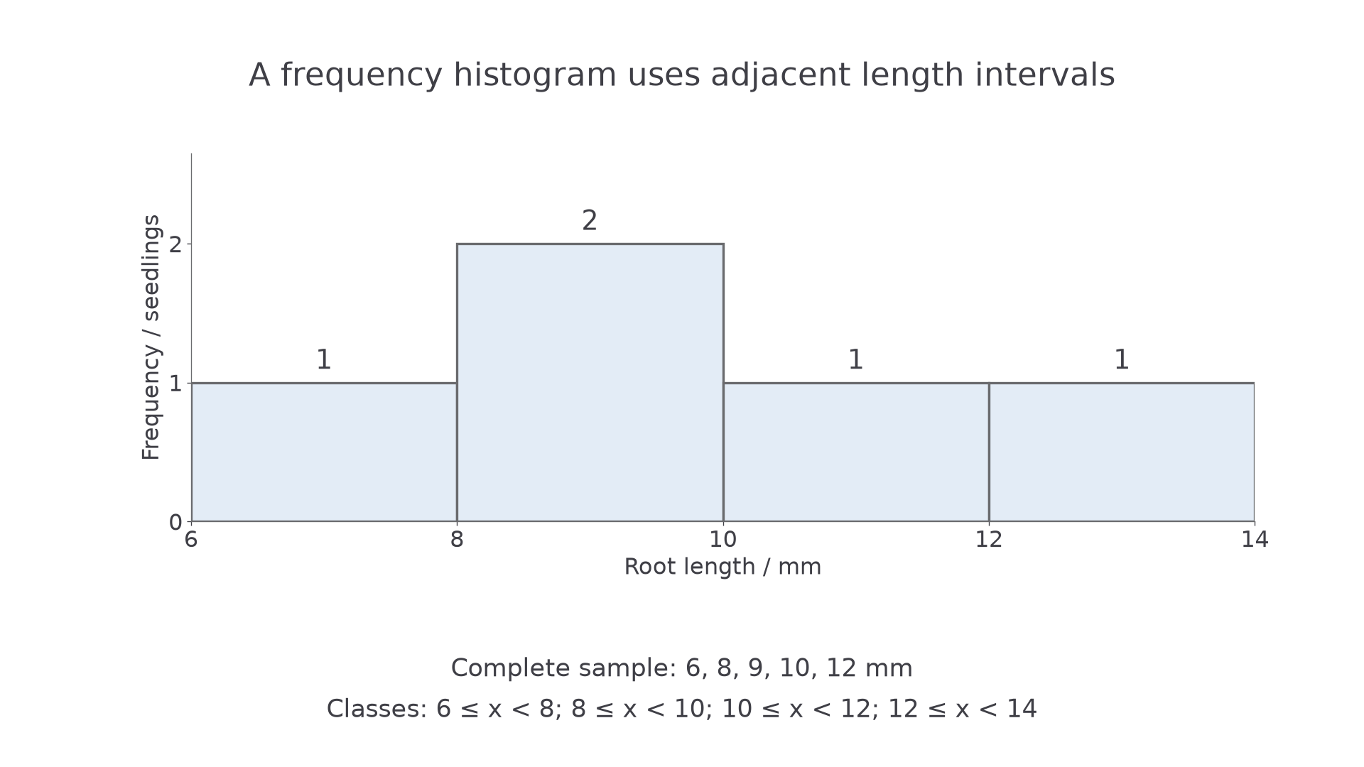
The 2 mm intervals touch because length is continuous. The modal class is 8–less than 10 mm; the grouped display alone does not identify an exact modal length.
To construct this histogram, put root length with its unit on the horizontal axis, mark the interval boundaries 6, 8, 10, 12 and 14, and draw adjacent bars of equal width with heights 1, 2, 1 and 1. With equal class widths, a frequency axis is appropriate. For unequal widths use frequency density, frequency divided by class width, so bar area, rather than height alone, represents frequency. A bar chart for separate categories, such as red-, white- and purple-flowered plants, instead has separated bars and a frequency axis; category widths do not represent a continuous measurement interval.
Grouping loses exact positions within each class. Retain raw measurements when calculating an exact mean, median or SD. Class midpoints can give an estimated mean, but it must be labelled an estimate. A small histogram can show this sample's distribution; it does not establish that the population has a normal distribution.
Calculating dispersion
Two samples can share a mean while differing greatly in how variable their individuals are.
Dispersion
Dispersion is the spread of values. The range is the largest value minus the smallest. Standard deviation, or SD, describes spread around the mean using all observations.
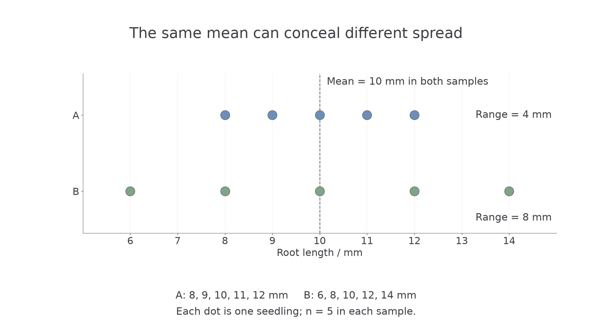
Both samples have mean 10 mm. A contains 8, 9, 10, 11 and 12 mm, whereas B contains 6, 8, 10, 12 and 14 mm. Their ranges are 4 and 8 mm respectively; each dot represents one seedling.
Range is quick, but it ignores where every non-extreme observation lies. SD includes all deviations, although its squared deviations give extreme observations a strong influence. SD can therefore be more informative than range when an extreme observation alone determines the range; it is not immune to outliers. Inspect the raw values or a plot alongside either summary.
A complete sample-SD calculation
Use the original five seedlings: 8, 9, 10, 10 and 13 mm. We treat them as a sample from a larger population and use the sample convention:
Here is an individual measurement, the sample mean, the number of observations, means add over all observations, and is sample SD. This formula requires at least two observations. SD has the same unit as the measurements.
The mean is . Subtract it from every length, square each deviation and add:
| / mm | / mm | / |
|---|---|---|
| 8 | −2 | 4 |
| 9 | −1 | 1 |
| 10 | 0 | 0 |
| 10 | 0 | 0 |
| 13 | 3 | 9 |
| Sum | 0 | 14 |
The deviations sum to zero, so averaging signed deviations would hide spread. Squaring prevents that cancellation. Divide the squared-deviation total by , obtaining sample variance ; then take the square root:
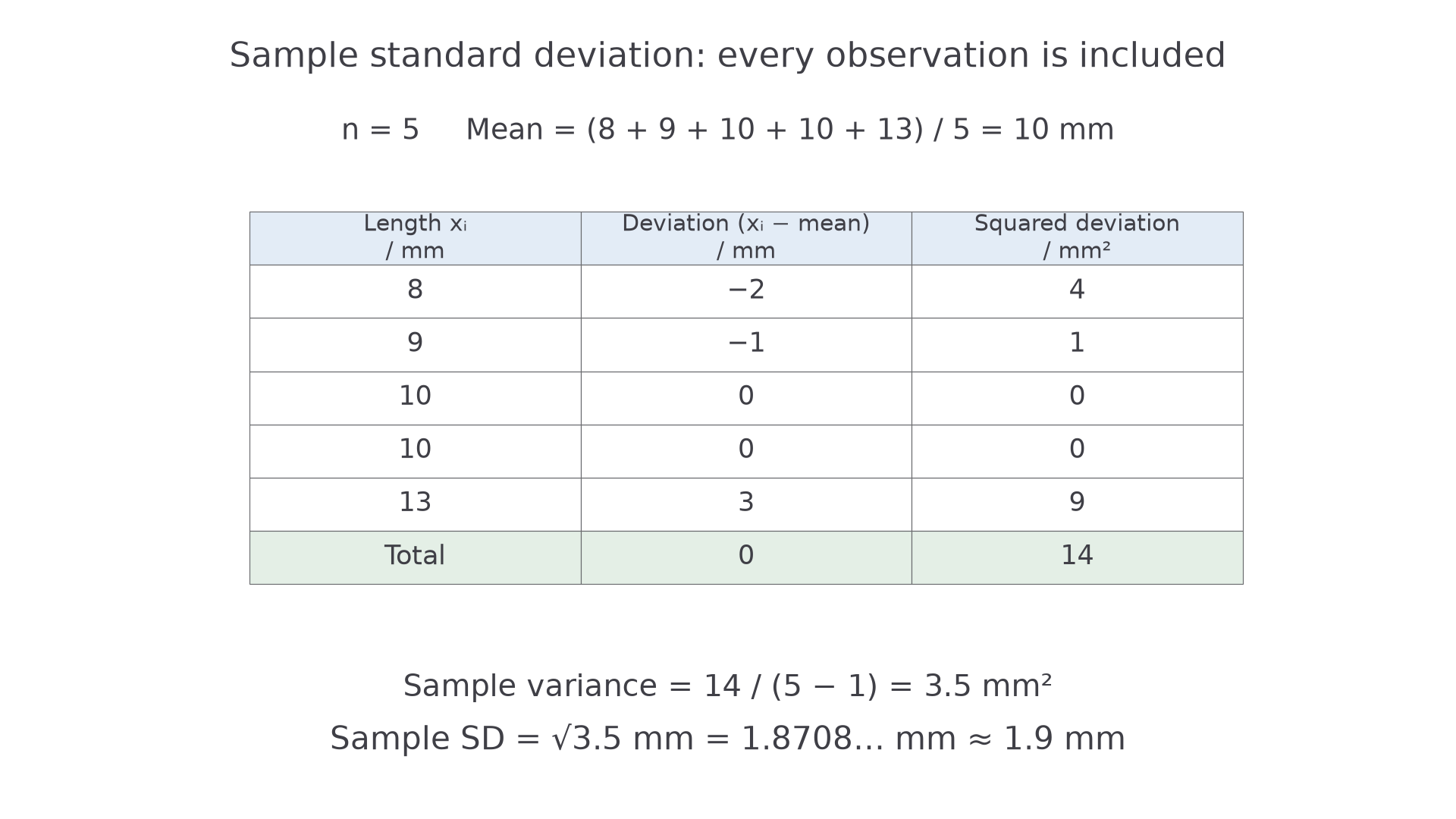
The denominator is four, because five observations are used with a mean estimated from those observations. Taking the square root restores millimetres.
The denominator accounts for estimating the population mean with the same sample: after the mean is fixed, only deviations can vary freely. The formula with denominator instead describes the population-SD convention when the values constitute the whole population of interest. Follow the stated convention; on a calculator the sample function is often labelled , whereas often uses . Check the calculator's definition rather than its symbol alone.
For these roots the range is . Replacing 13 by 23 mm changes the range to 15 mm and sample SD to about 6.2 mm, as well as changing the mean to 12 mm. Investigate a possible outlier: check the original record, instrument, sample identity and procedure. A documented transcription mistake should be corrected transparently; a genuine biological extreme should not be deleted merely to obtain a smaller SD or a preferred conclusion.
Uncertainty and errors
Variation between organisms and variation in the way we measure one organism are different sources of spread.
Genetic and environmental differences can give different seedlings different root lengths. Repeatedly measuring the same root, while its length is unchanged, instead helps reveal variation in measurement. Readings 19.9, 20.0, 20.0 and 20.1 mm have mean 20.0 mm and range 0.2 mm. Half that range, 0.1 mm, is a simple description of the observed repeat scatter in this small example; it is not automatically a complete uncertainty estimate. Four repeats may miss wider variation and cannot reveal every calibration problem.
Measurement uncertainty
Measurement uncertainty describes the doubt associated with a reported measurement, taking account of the method and relevant information. It is not the exact error, which would require knowing the true value, and it is not a licence to include avoidable mistakes.
Distinguish the following when deciding what an improvement would achieve:
| Idea | Meaning and root-measurement example | Useful response |
|---|---|---|
| Random error | Unpredictable variation between readings, for example varying judgement of a blurred root tip | Standardise the endpoint; repeat measurements and examine their scatter. Averaging independent, unbiased errors can reduce their contribution to a mean. |
| Systematic error | A consistent bias under the conditions, for example a ruler's displaced zero making every length too large | Compare with a suitable calibrated reference and correct the bias or change the method. More repeats alone do not remove it. |
| Mistake | An avoidable blunder, such as copying 21 mm as 12 mm or using the wrong unit | Check and correct the record with an audit trail; do not treat the mistake as ordinary uncertainty. |
| Accuracy | Closeness to the true or accepted reference value | Assess calibration and relevant bias; closely agreeing readings alone cannot demonstrate accuracy. |
| Precision | Closeness of repeated readings to one another under stated conditions | Inspect repeat scatter. A narrow scatter can coexist with systematic bias. |
Resolution is the smallest change the instrument can distinguish. A display with more decimal places has finer resolution, but that does not by itself establish better accuracy. Parallax, a poorly defined endpoint, calibration and changing conditions may matter more than the last digit. An error may also arise from the sampling or experimental design: measuring more leaves from only one plant does not necessarily represent a whole habitat better.
Before reporting uncertainty, identify the quantity being measured and the important sources. Correct known significant biases where possible and retain uncertainty about the correction. Repeats help assess random variation, but biological replication and instrument calibration answer different questions. There is no general rule that every uncertainty decreases by dividing by the number of repeats or by its square root.
Absolute and percentage uncertainty
An uncertainty needs a value, a unit and an explanation of what its limits mean.
Continue this lesson.
You’re previewing NovaLearn without an account. Create a free account to read the rest.
Create free account