5.14 - Climate models and predictions
Climate evidence describes changes that have already happened; models help us investigate what could happen next. You will use a simple straight line to make and check a prediction, then distinguish that exercise from physical climate models and explain why useful projections still have limits.
Extrapolation and conditional projections
A pattern within existing data can suggest what may happen beyond the measured interval, provided its assumptions remain reasonable.
Extrapolation
Estimating a value outside the range of the available data by extending an assumed relationship.
Estimating a value between two measured dates is interpolation. Extending a temperature trend from measurements ending in 2020 to estimate a value in 2040 is extrapolation. The calculation may be correct while the prediction fails if the relationship changes. A short interval dominated by an unusual warm or cool fluctuation is particularly weak evidence for a persistent rate.
For future climate, scientists investigate different scenarios: explicit assumptions about future drivers, such as greenhouse-gas emissions, aerosols and land use. Observed trends and extrapolated assumptions about these drivers can inform future model inputs. The model then calculates the climate response; it does not simply extend every observed temperature graph with a ruler.
Climate projection
A simulated future climate response conditional on stated assumptions, including an emissions scenario.
A forecast or prediction aims to describe what will actually occur. A scenario projection asks what would follow if its assumptions occurred. This distinction matters because future emissions depend on human choices. A scenario is not assigned a probability merely because it appears on a graph. Climate projections usually concern statistics such as average temperature or the frequency of hot days over an interval, rather than the exact weather on a particular distant date. The Met Office explains the scenario approach.
Physical models, inputs and feedback
A physical climate model represents interactions among the atmosphere, ocean, land and ice using mathematical relationships based on physical principles, including conservation of energy.
In a global circulation model, calculations are made on a three-dimensional grid and repeated through time. Radiation changes the energy balance; winds and ocean currents redistribute energy; water evaporates, condenses and falls as precipitation. Inputs and boundary conditions describe factors such as greenhouse-gas concentrations, aerosols, solar energy and the land surface. Some models take emissions and calculate concentrations using carbon-cycle processes. Measurements help establish the starting state and test the simulated climate. NCAS describes how these models operate.
An initial change can also trigger feedback: a response that changes the original effect. Warming can reduce snow and sea-ice cover. A darker exposed surface reflects less sunlight and absorbs more, reinforcing warming: a positive feedback. “Positive” means amplifying, not beneficial. Increased outgoing thermal radiation as temperature rises opposes the initial warming, a negative feedback. Clouds affect both reflected sunlight and outgoing thermal radiation; representing their responses is one source of uncertainty. Feedback therefore changes the size of the response to an imposed driver. The Met Office connects feedback with climate sensitivity.
Models simplify processes smaller than their grid cells using approximate relationships. Finer grids can represent more detail but require more computing. Adding detail is valuable when it improves the model's tested performance for the intended question; complexity alone is not proof of accuracy.
A local linear fit and extrapolation
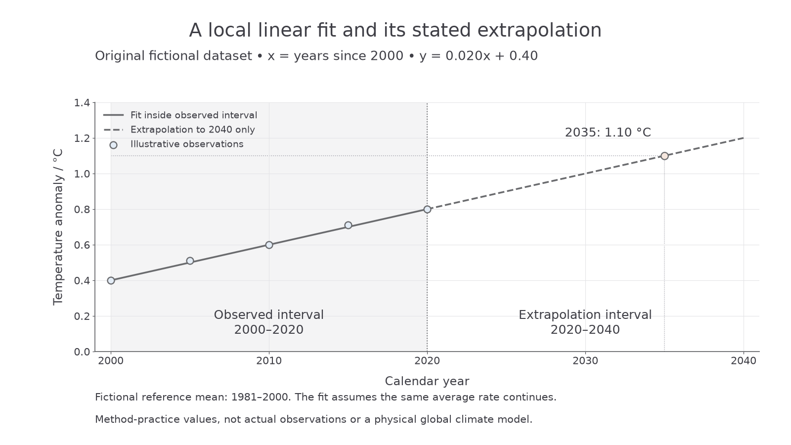
A straight-line exercise makes the assumptions behind extrapolation visible, but it is much simpler than a physical climate model.
The following is a complete original fictional dataset for learning the method, not measured global temperature data. Its temperature anomaly is a difference from a fictional 1981–2000 reference mean. For example, an anomaly of +0.40 °C means 0.40 °C above that reference, not an absolute temperature of 0.40 °C.
| Calendar year | , years since 2000 | Illustrative observed anomaly / °C |
|---|---|---|
| 2000 | 0 | 0.40 |
| 2005 | 5 | 0.51 |
| 2010 | 10 | 0.60 |
| 2015 | 15 | 0.71 |
| 2020 | 20 | 0.80 |
The values increase by about 0.10 °C in each five-year interval and lie within 0.01 °C of a straight line. That supports a local linear approximation over 2000–2020. It does not establish that the same trend must continue indefinitely. We choose a transparent line through the first and last values, rather than claiming to have performed a statistical regression.
For a linear relationship, .
Here , , and is time in years since 2000.
Thus , with in °C.
The slope means the fitted anomaly rises by 0.020 °C each year, or 0.20 °C per decade. The intercept is the fitted anomaly at , which here means calendar year 2000. It is not the anomaly in calendar year zero. Changing the time origin would change the intercept; it would not change this fitted rate.
Estimate, calculate and check
Suppose we explicitly allow this simple exercise to extrapolate only from 2020 to 2040, assuming the average rate remains constant. Estimate the 2035 anomaly first: 2035 is 15 years after 2020, so a rise of roughly three lots of 0.10 °C gives about 1.1 °C. Now substitute the correct time coordinate, :
The calculation agrees with the estimate. The positive sign, units and scale make sense. The two decimal places describe the exercise's numbers, not knowledge of real 2035 climate to 0.01 °C. A graph reading at 2015 is interpolation within the observed interval; the 2035 result is extrapolation 15 years beyond its end. Neither the equation nor our stated range authorises a prediction for 2100. The chosen 2040 endpoint is a practice boundary, not a scientifically established safe prediction horizon.
Continue this lesson.
You’re previewing NovaLearn without an account. Create a free account to read the rest.
Create free account