5.12 - Evidence for climate change
Climate evidence comes from instruments and from natural records that preserve clues about the past. In 5.12 you will interpret carbon dioxide and temperature records, pollen in peat bogs and tree rings, then distinguish a correlation from evidence about a cause.
Temperature records and climate
A cold winter describes conditions over a short period; a climate claim concerns the longer-term pattern of conditions, including averages and variability.
Weather is the short-term state of the atmosphere. Climate describes its statistical pattern over longer periods, often using 30-year averages. A single cold day, place or year can occur within a warming climate. Assess a trend across a suitable interval and area rather than selecting one unusually warm or cold endpoint. NOAA explains this weather–climate distinction.
Thermometers at land stations and measurements of sea-surface temperature from ships and buoys provide instrumental records. Instruments need calibration against standards. Station moves, altered instruments and changes in measurement practice can introduce jumps unrelated to climate; documented checks and comparisons with nearby records help identify these. Global estimates also need spatial weighting: a densely monitored region must not count more merely because it has more stations. Sparse early coverage increases uncertainty.
Temperature anomaly
The difference between a temperature and the average for a stated reference period. A positive anomaly means warmer than that reference, not a temperature above zero degrees Celsius.
For a local temperature record, this relationship translates the definition into algebra.
Here is the anomaly, the temperature and the reference-period mean for that location and time of year. Use the same temperature units throughout.
For a simple local example, if a station's annual mean is and its reference mean is , the anomaly is . Keeping the same reference makes changes comparable. NASA GISTEMP combines local anomalies into an area-weighted global index, rather than simply averaging every station's absolute temperature. Its reference is 1951–1980. Changing a fixed baseline shifts anomaly values but does not reverse the underlying trend. NASA GISS describes its measurements and processing.
An instrumental temperature record measures the changing temperature outcome. On its own it does not identify which influence caused the change. Long coverage, many locations, consistent processing and agreement among different observations strengthen the evidence.
Carbon dioxide and instrumental trends
Carbon dioxide records measure atmospheric composition, which can be compared with temperature records but is a different variable.
Modern analysers measure the proportion of carbon dioxide in air. Parts per million, or ppm, expresses the number of carbon dioxide molecules per million molecules of dry air. A concentration is not an emission rate: emissions add carbon dioxide, while exchange with oceans and land also affects how much remains in the atmosphere. A background-air record such as Mauna Loa is valuable, but one site is not itself a global mean. Comparisons across the wider monitoring network test whether a change is widespread. NOAA publishes the Mauna Loa record and its measurement information.
For older periods, air enclosed in polar ice preserves samples of past atmospheric gases. Scientists extract this air and measure its carbon dioxide concentration. Dating the archive is essential: snow remains porous before air is sealed into bubbles, so the enclosed air and surrounding ice need not have the same age. Gas trapping also smooths rapid variations. Comparisons require appropriate gas-age estimates, not the assumption that equal core depths mean exactly simultaneous events. British Antarctic Survey reviews ice-core carbon dioxide methods.
The following are real selected annual means, downloaded from NOAA GML and NASA GISS on 15 October 2026. They are one year per decade, not decade means. NASA values are global temperature anomalies relative to 1951–1980; the carbon dioxide values are Mauna Loa annual means.
| Year | Carbon dioxide / ppm | Global temperature anomaly / °C |
|---|---|---|
| 1960 | 316.91 | −0.02 |
| 1970 | 325.68 | +0.03 |
| 1980 | 338.76 | +0.26 |
| 1990 | 354.45 | +0.45 |
| 2000 | 369.71 | +0.39 |
| 2010 | 390.10 | +0.72 |
| 2020 | 414.21 | +1.01 |
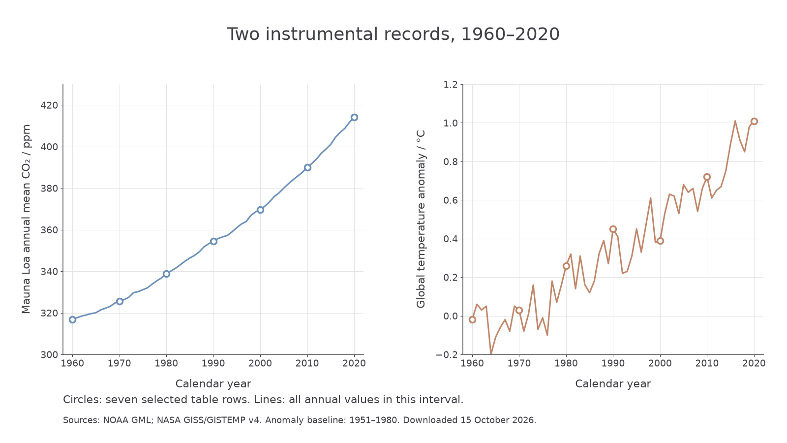
The lines show all annual values in 1960–2020; circles identify the seven table rows. Sources: NOAA GML and NASA GISS/GISTEMP v4. These are separate axes with different units, not two interchangeable scales.
A time-series graph puts year on the horizontal axis and the measured quantity on the vertical axis. Locate 2010, move vertically to the carbon dioxide circle, then horizontally to its scale: the table gives , read approximately as at this graph's scale. In the temperature panel, 2010 gives approximately . Thus a pair of graph readings can be returned to a numerical row. Do not claim more decimal precision from a graph than its scale permits.
From the table, carbon dioxide rose by between 1960 and 2020. The anomaly difference is . This means the global index was 1.03 °C warmer in the later selected year, not that its absolute temperature was 1.03 °C. These endpoints summarise a change; the complete annual curve reveals the fluctuations between them.
Pollen in dated peat
Pollen preserved in peat provides evidence about past vegetation, from which past climate can be inferred.
Peat accumulates where waterlogged conditions restrict decomposition. Pollen grains deposited from surrounding vegetation can survive because their outer walls resist decay. In a relatively undisturbed sequence, deeper layers are generally older. A core preserves this order: samples from successive depths are examined microscopically, pollen types identified and their abundances counted. Some grains can be identified only to a family or genus, so the evidence does not always identify an exact species. USGS describes pollen preservation and identification.
Climate proxy
A measured feature that can be used to infer a past climate variable through an established relationship, rather than a direct reading of that climate variable at the time.
Plants have different tolerances of temperature and water availability. Comparing a fossil pollen assemblage with modern vegetation and measured climates helps interpret past conditions. The chain of inference is pollen assemblage → vegetation → likely environmental conditions. Pollen is not a direct thermometer; the same vegetation pattern may be influenced by rainfall, soils, succession or land use. NOAA describes this use of fossil pollen.
Depth supplies a relative sequence, not a calendar date. Radiocarbon measurements of suitable organic material at several depths, calibrated to calendar ages, can anchor an age–depth model. Ages between dated levels are estimates; peat accumulation can vary, and disturbance or contamination can complicate the sequence. Several centimetres may represent many years, so a short event can be blurred or missed. A USGS peat study illustrates radiocarbon dating and estimated pollen-zone ages.
This original illustrative dataset is invented for learning the method. The ecological groups and ages below do not represent a real bog. In this example, modern comparisons associate the woodland group with warmer conditions and the open-vegetation group with colder conditions, subject to other environmental influences. Each row totals 100% of counted pollen; percentages are not necessarily the percentage of ground covered by each plant group.
| Calibrated age / years BP | Warmth-associated woodland pollen / % | Cold-tolerant open-vegetation pollen / % | Other pollen / % |
|---|---|---|---|
| 6000 | 10 | 70 | 20 |
| 4500 | 25 | 55 | 20 |
| 3000 | 50 | 30 | 20 |
| 1500 | 60 | 20 | 20 |
| 500 | 55 | 25 | 20 |
BP here means years before 1950. A pollen diagram can plot percentage horizontally and age vertically, with older ages lower down. Plotting the woodland pair and then shows a large shift toward woodland pollen as time advances. Read the axes carefully: moving upward means moving toward more recent ages. This change supports warmer local conditions between those levels, given the supplied ecological relationship; it does not yield an exact temperature or prove that temperature alone changed. The small reversal at 500 BP should also be reported.
Different plants produce and disperse different amounts of pollen, and some pollen travels a long way. A bog samples a particular source area, not the whole planet. Several cores and independent proxies help check whether a pattern is regional. A real NOAA-archived reconstruction used multiple peat-bog pollen sequences, modern pollen and meteorological calibration, and radiocarbon dates; its target was rainfall, showing why the climate variable must be justified rather than assumed to be temperature. Original reconstruction metadata.
Continue this lesson.
You’re previewing NovaLearn without an account. Create a free account to read the rest.
Create free account