5.3, Core practical 10 - Niches, quadrats and transects
A plant may grow abundantly beside one part of a path and be absent a few metres away. In 5.3, you will use its niche to explain such patterns; in Core practical 10, you will design a habitat study, identify organisms, sample their distribution and abundance, and measure relevant abiotic conditions. The aim is to build a defensible biological explanation from field evidence while recognising what a survey cannot establish.
Niches and field hypotheses
An organism's habitat is where it lives, whereas its niche describes how it lives there.
Niche
The ecological role of a species, including the resources it uses, the environmental conditions it tolerates and its interactions with other organisms.
A ground plant needs suitable light, water, mineral ions and temperature to maintain metabolism, grow and reproduce. Its distribution is the pattern of places where it occurs; its abundance is how much of it occurs. A species can be absent where a condition exceeds its tolerance, or scarce where conditions permit survival but restrict reproduction. Conditions that support rapid growth can allow abundance to increase, provided seeds reach the site and biotic interactions permit establishment.
For example, a shade-tolerant plant may survive beneath a canopy where a plant with a higher light requirement cannot maintain sufficient photosynthesis. In an opening, greater light may favour a fast-growing competitor, which shades the first plant. Grazing, disease and competition can therefore restrict a species even within its physical tolerance range. Availability of suitable conditions alone does not guarantee its presence: dispersal, season and past disturbance also matter. A niche is more than a position on one light gradient.
Translate this explanation into a measurable question: “Does the percentage cover of ground-plant species S change with distance from the woodland edge, and how does cover relate to measured light?” A directional hypothesis might predict lower cover of S farther into the open area if S is associated with shaded conditions. State the biological reason before collecting data. Distance is a position variable; it is not itself the mechanism affecting growth. Light and soil moisture may both change with distance.
Choose a response that can actually be measured. Quadrat counts suit distinct, rooted rosettes; percentage cover suits a spreading plant whose individuals cannot be separated confidently. Quadrat methods are poorly suited to estimating fast-moving animals that escape or enter during counting. The question, organism and method must fit one another.
Identification and supporting techniques
A precise count of the wrong species is still an invalid abundance estimate, so establish identification before the main survey.
Use a current field guide or an appropriate identification key. A key offers contrasting observable features, such as leaf arrangement, leaf shape and flower structure; follow each choice to an identification rather than choosing the most similar photograph. Practise on known specimens, record the guide's title/edition or website and access date, and agree species codes across the group. A hand lens may reveal diagnostic hairs. Photograph uncertain specimens with a scale and record their coordinates; seek confirmation and retain an “unidentified” category until resolved. Do not silently assign an uncertain specimen to the expected species. Different life stages or missing flowers can limit a key's usefulness.
Where microscopic features are relevant, a supervised laboratory preparation can support identification. Place permitted plant material in a water drop on a slide, lower a coverslip at an angle to reduce bubbles, and locate the specimen at low power. Centre and focus it before changing to high power; use fine focus at high power to avoid driving the objective into the slide. A microscope does not automatically distinguish all species, so compare a diagnostic feature with a reliable reference.
An eyepiece graticule has arbitrary divisions. Calibrate it against a stage micrometer at each objective used. If 40 graticule divisions span 100 micrometres on the stage scale, one division represents . An observed feature spanning 8 divisions is . Changing objective invalidates that calibration. Make a large, clear scientific drawing from the actual observation with single outline strokes, no invented structures or decorative shading, ruled label lines, a title and a calibrated scale bar or stated magnification. An annotation should explain an observed feature's significance; a drawing copied from a guide is not a record of your specimen.
Qualitative reagents can support a separate biological question arising from a habitat study. For example, in a supervised laboratory, add iodine solution to teacher-prepared decolourised leaf material to test for starch, alongside a known starch suspension and a water negative control. Blue-black staining is positive; iodine remaining yellow-brown is negative. Use labelled small quantities, eye protection and the centre's reagent-handling/disposal instructions. If fresh leaves need decolourising, the teacher manages the hot ethanol preparation: ethanol is flammable and must not be heated over a flame. A starch result identifies a biological molecule; it does not identify the species or establish that light caused its field distribution. The controls check the reagent response, not the survey's sampling validity.
These are concrete opportunities to prepare microscope, observation/drawing and molecule-test skills alongside field identification. They should be used when relevant and permitted, rather than added destructively to every quadrat. Teacher observation of real apparatus use, individual decisions and contemporaneous records is necessary for practical competence; reading or answering online cannot authenticate the centre's CPAC endorsement.
Random quadrats and abundance
Random quadrats estimate abundance across a defined area without deliberately favouring conspicuous plants or convenient patches.
Before sampling, obtain access permission, define the study boundary and target species, and pilot a practical frame size. Here a 0.50 m by 0.50 m frame encloses , because 50 cm is 0.50 m and area uses the square of the length conversion. Check the frame's internal dimensions. A tiny frame may miss a patchy plant; a huge one may take too long to identify consistently. Use the same area and observation rules throughout comparisons.
For this original practice example, a 10 m by 10 m grassland plot is divided into 400 non-overlapping 0.50 m square cells. Mark two perpendicular tapes from a fixed origin. Generate pairs of integers from 0 to 19 uniformly, without replacement. The lower-left corner of the selected cell has coordinates , metres. Every equal-area cell has the same chance of selection and every selected frame fits inside the boundary. Locate cells from the tapes; do not throw a quadrat or move it to include an interesting plant. Predefine any inaccessible exclusions and the corresponding target area before drawing coordinates. Keep the random list and any justified replacement records. This adapts the coordinate-based approach described by the Field Studies Council to equal-area cells with an explicit boundary rule.
For countable plants, count rooted individuals, not flowers or leaves. Set a boundary rule in advance: include roots on the top and left edges, exclude those on the bottom and right. This prevents double counting without choosing case by case. For spreading vegetation, estimate the vertical projection covering the frame using a grid; count fully covered cells and combine partial areas. If 28 whole cells plus partial areas equivalent to 7 cells are covered in a 100-cell grid, estimated cover is 35%. Repeat observers can agree a protocol using practice quadrats before data collection. Species can overlap vertically, so covers of different species need not sum to 100%. Cover is not a count of individuals.
The table gives the complete original teaching dataset. It is constructed practice data, not measurements from a claimed field visit. Clover cover is estimated to the nearest 5 percentage points.
| Quadrat | Lower-left / m | Daisy rooted individuals | Clover cover / % |
|---|---|---|---|
| 1 | (1.0, 2.0) | 4 | 10 |
| 2 | (4.5, 7.0) | 0 | 0 |
| 3 | (7.0, 1.5) | 7 | 30 |
| 4 | (2.5, 8.5) | 3 | 20 |
| 5 | (6.0, 5.5) | 5 | 15 |
| 6 | (8.5, 3.0) | 0 | 0 |
| 7 | (3.5, 4.0) | 8 | 35 |
| 8 | (5.0, 0.0) | 2 | 10 |
| 9 | (0.0, 6.5) | 6 | 25 |
| 10 | (7.5, 8.0) | 1 | 5 |
| 11 | (9.0, 5.0) | 0 | 0 |
| 12 | (4.0, 3.0) | 6 | 30 |
Density has units such as individuals per square metre. Percentage frequency is a presence/absence measure for the stated quadrat size.
There are 42 daisies in . Mean count per quadrat is ; density is . Daisies occur in 9 of 12 quadrats, so frequency is 75%. Cover totals 180 percentage points across the 12 observations, giving mean clover cover . Do not divide the count by the entire 100 square metre plot: most of that area was not counted. Estimated total daisies in the target plot would be , conditional on representative sampling; it is not an exact census. Frequency cannot distinguish one daisy from eight in a quadrat and changes if quadrat size changes.
Twelve samples make this example manageable, but do not guarantee adequacy. Use pilot variation, habitat patchiness and the study's desired precision to plan effort; increase dispersed samples and inspect how estimates and their variation change. Rare species may require greater effort. If distinct zones occupy different proportions, use proportionate random sampling within zones or analyse zones separately before a correctly weighted estimate. Many adjacent subsamples in one patch do not represent independent coverage of the whole plot.
Transects across a gradient
A transect deliberately follows an environmental gradient to reveal how distribution and abundance change with position.
For the woodland question, place a tape from the edge towards the open grassland, perpendicular to the edge. A line transect records organisms touching the line at stated positions. A belt transect samples a strip using quadrats: contiguous frames make a continuous belt, while separated stations make an interrupted belt. Use a continuous belt where narrow changes would be missed by large gaps; an interrupted belt trades spatial detail for coverage over a longer distance.
Preselect a suitable interval from a pilot, rather than adjusting stations to find S. In the worked design, place the same 0.50 m square frame on the same side of the tape, with its lower-left corner at 0, 4, 8, 12, 16 and 20 m. Record S cover and relevant abiotic readings at each station. The fixed placement convention matters: moving frames to avoid bare ground would bias cover upward. Standardise frame size, identification/cover method, sensor position and timing. In a field survey, other abiotic variables usually cannot be held constant; measure important alternatives rather than claiming to have controlled the weather or soil.
Use several separately positioned transects with randomly selected starting positions along the available edge, with preplanned spacing sufficient to avoid overlapping quadrats and to reduce dependence between local patches. The exact worked layout below has transects T1, T2 and T3 at lateral positions 0, 5 and 10 m; actual field spacing must reflect the habitat's patch size. Three readings at different stations of one line are not three independent woodland sites. Replication across separately located lines improves evidence for that edge; replication across separate woodlands is needed before broad claims about woodlands generally. Sampling at different times can reveal seasonal or daily variation, but temporal readings also have their own dependence.
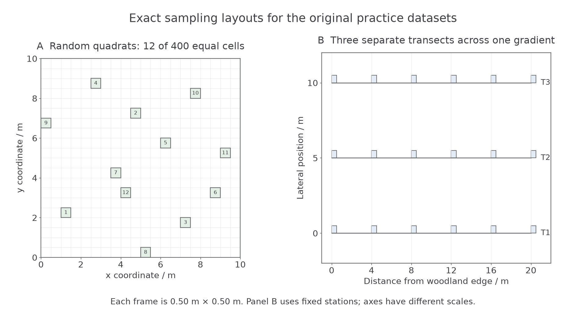
The original practice layouts show the 12 selected equal-area cells on the left and three transects with fixed 4 m station intervals on the right. Each frame is 0.50 m square; the right panel's horizontal and vertical axis scales differ.
The following complete original practice records refer to the three transects. Each cover estimate is to the nearest 5 percentage points. Illuminance readings in kilolux are supplied for analysing the association, not as a claim that lux measures photosynthetic photon flux directly.
| Distance / m | S cover T1 / % | S cover T2 / % | S cover T3 / % | Illuminance T1 / klx | Illuminance T2 / klx | Illuminance T3 / klx |
|---|---|---|---|---|---|---|
| 0 | 70 | 60 | 80 | 1.0 | 1.2 | 0.8 |
| 4 | 60 | 55 | 65 | 2.0 | 2.2 | 1.8 |
| 8 | 45 | 40 | 50 | 4.0 | 4.2 | 3.8 |
| 12 | 30 | 25 | 35 | 6.0 | 6.2 | 5.8 |
| 16 | 15 | 10 | 20 | 8.0 | 8.2 | 7.8 |
| 20 | 5 | 0 | 10 | 10.0 | 10.2 | 9.8 |
Abiotic measurements and field care
Abiotic readings are useful only when they represent the conditions experienced by the sampled organisms and can be compared consistently.
Select factors for a biological reason. Ground-level light may affect a ground plant's photosynthesis; soil moisture affects water supply; pH affects nutrient availability. In freshwater, temperature, dissolved oxygen and flow may be more appropriate. You do not need to use every available instrument at every site.
| Quantity | Feasible measurement | Calibration or consistency check |
|---|---|---|
| Illuminance / lux or klx | Light meter or logger at a fixed height just above the vegetation, facing the same direction | Use a suitable range, check zero/cover response and manufacturer calibration; compare matched meters together. Do not shade the sensor with your body. |
| Soil temperature / degrees Celsius | Digital temperature probe at a stated depth, allowing the reading to stabilise | Check against a reference thermometer or an appropriate known-temperature check; use equal depth and equilibration time. |
| Soil pH / no unit | A pH probe in a consistent soil–distilled-water suspension | Calibrate with suitable known buffer solutions, rinse between samples and read after stabilisation; keep soil:water ratio and mixing time constant. |
| Soil moisture / defined % | A soil-moisture probe, or a permitted small soil sample measured by mass loss on drying | A probe requires a soil-appropriate calibration before calling output a water percentage; retain the actual units if it gives only an index. |
| Wind speed / metres per second | Anemometer at a fixed height for a fixed measurement interval | Check operation and manufacturer requirements; retain averaging interval and avoid sheltering it with an observer. |
Continue this lesson.
You’re previewing NovaLearn without an account. Create a free account to read the rest.
Create free account