6.1 - Estimating time of death
After a mammal dies, its temperature, muscles and communities of decomposers change. These changes provide different kinds of evidence about elapsed time. Learn how to interpret them together, use temperature and insect-development graphs, and explain why a defensible estimate usually gives a range rather than an exact moment.
Elapsed time and biological evidence
An investigator observes a body at a known time, but biological processes do not all begin together or run at a constant rate. A good estimate identifies what each observation measures before converting it into a possible time of death.
Post-mortem interval
The post-mortem interval (PMI) is the elapsed time between death and a specified later observation, such as discovery or examination.
If discovery is at 15:00 and the estimated PMI is 5–7 hours, the possible death interval is 08:00–10:00 that day. Subtract the longer elapsed time to find the earlier clock time. Keep the date when an estimate crosses midnight.
For a stated observation time, estimated time of death = observation time − estimated PMI. Use matching time units and carry any estimated interval through the subtraction.
Each biological process has its own course, and overlapping processes do not form one universal timetable:
| Evidence | Biological change being interpreted | Important qualification |
|---|---|---|
| Body temperature | Change in stored thermal energy after effective thermoregulation stops | Depends on starting temperature and heat exchange with the surroundings |
| Degree of muscle contraction | Development and later loss of post-mortem stiffness | Absence of stiffness can occur before or after rigor |
| Extent of decomposition | Enzymatic and microbial breakdown of tissues | Rate depends strongly on conditions |
| Stage of succession | Changes in the organisms associated with the remains | Needs comparison with a suitable local habitat and season |
| Forensic entomology | Identity and development of insects associated with the remains | Usually dates colonisation or development, with assumptions needed to infer death |
The next parts explain why these qualifications matter. A number obtained from a graph is conditional on the biological model and the observations used to build it.
Decomposition and community succession
Decomposition changes both the tissues and the food resources available to other organisms. Autolysis is breakdown by the body's own enzymes after normal cellular control is lost. Microorganisms also use enzymes to break down organic material; their metabolism changes the chemical environment. Feeding insects and other consumers contribute to tissue loss. These processes overlap.
Observers commonly describe fresh, bloated, active-decay, advanced-decay and dry-remains stages: a progression from few visible changes, through increasing microbial activity and gas production, to substantial tissue breakdown and eventually predominantly dry material. These are descriptions of condition, not assigned numbers of days. Different regions of one body can change at different rates, and drying or cold can interrupt the usual progression.
Succession on remains
Succession is a change in the composition of the associated community over time as resources and environmental conditions change.
Early colonisers, such as blowflies in many exposed terrestrial settings, can use moist, accessible resources. Their feeding and the activity of microorganisms alter those resources. Some later insects, including particular beetles, feed on drier material, while predators or parasites may exploit insects already present. A controlled succession study found early fly dominance and later increases in beetles, but also variation between studies at the same location. The species present, their relative abundance and the condition of the remains can therefore be compared with observations from known-time decomposition studies. The particular sequence varies with geography, habitat and season; no one insect species always means a fixed number of days.
| Changed condition | Why the same elapsed time may give different evidence |
|---|---|
| Lower temperature | Many enzymatic reactions, microbial processes and insect development proceed more slowly within their normal operating range |
| Very dry conditions | Water becomes limiting and material can dry rather than follow the same decay pattern as moist remains |
| Burial, enclosure or covering | Access by particular insects, oxygen supply and the local temperature/moisture may change |
| Different mammal size or condition | Available resources, insulation and tissue characteristics differ |
| Scavenging or movement | Material or insect evidence may be removed, or a body may acquire evidence from more than one location |
For example, a community dominated by insects associated locally with dry material can support a later stage of decomposition. It does not alone identify the death date: unusually dry conditions may have changed both the rate of breakdown and which species could live there. Research in one habitat cannot simply be transferred to a different climate. Field research on decomposition demonstrates why temperature and rainfall belong in the interpretation.
Insect age and colonisation
Forensic entomology uses insect evidence in an investigation. Developmental evidence asks how long a particular insect has been developing; succession evidence asks which community has assembled. These related approaches measure different things.
In an egg-laying fly, an egg hatches into a larva. Larvae pass through growth stages called instars, then enter a pupal stage before an adult emerges. A species may be recognised from suitable body features or laboratory identification. Developmental stage, and sometimes length within a specified growth phase, can be compared with species-specific experimental data. Length alone is insufficient: a later, non-feeding larva can shorten, so an arbitrary length is not a unique age across the whole life cycle.
Temperature affects the rate of development. Within a suitable range, warmer conditions usually allow a given stage to be reached sooner, but extreme temperatures can inhibit development or kill the insect. A specialist therefore needs the species, life stage and relevant temperature history, rather than only the air temperature at discovery. Direct sunlight, shade and heat produced by a mass of feeding larvae can make the actual microclimate differ from a distant weather station. Populations of the same species can also differ in development, so the calibration needs appropriate validation. NIJ's account of experimental development research supports this caution.
Investigators seek the oldest reliably identified developmental evidence, which may include pupae as well as larvae, and document where and when it was collected. Missing the oldest insects makes the inferred colonisation too recent. Continued development between collection and examination must also be accounted for; preserving representative specimens and rearing others under recorded conditions can help identify the species and stage. Research on delayed insect sampling shows why this interval matters.
Insect age usually supports a minimum PMI, conditional on colonisation having occurred after death. It dates development since egg laying or another specified life-stage event, not necessarily death itself. Restricted access, unsuitable weather or delayed arrival can make death earlier than the insect estimate; infestation that began before death would invalidate the usual assumption.
For instance, three days of insect development does not prove death occurred three days ago. If flies could only enter a room after a window opened, development may date access and subsequent colonisation instead. A complete reconstruction needs both biological development and evidence about when access was possible.
Plotting and reading insect development
A graph makes temperature-dependent development easier to compare, provided its starting event is stated. The following values are original fictional teaching data for Species X, not measurements from a real species or a usable forensic calibration. They describe only its feeding-larval growth phase under constant temperatures.
| Age after hatching / h | Length at 18 °C / mm | Length at 24 °C / mm |
|---|---|---|
| 0 | 2 | 2 |
| 12 | 3 | 5 |
| 24 | 5 | 9 |
| 36 | 8 | 13 |
| 48 | 11 | 15 |
| 60 | 13 | 16 |
| 72 | 14 | 17 |
To plot these two variables, put age after hatching on the horizontal axis and larval length on the vertical axis. Use a linear horizontal scale from 0 to 72 h, for example 6 h per major division, and a vertical scale from 0 to 18 mm, for example 2 mm per major division. Label both axes with quantities and units. Plot each coordinate accurately: at 24 h, one point is (24, 5) for 18 °C and the other is (24, 9) for 24 °C. Use distinct symbols and a key for the two temperatures. For this exercise, join consecutive points with straight segments to permit local interpolation; do not extrapolate beyond the stated feeding phase.
Make the graph yourself on paper or with a suitable plotting tool before comparing it with the completed graph. A written description of plotting is not evidence that the points were actually plotted.
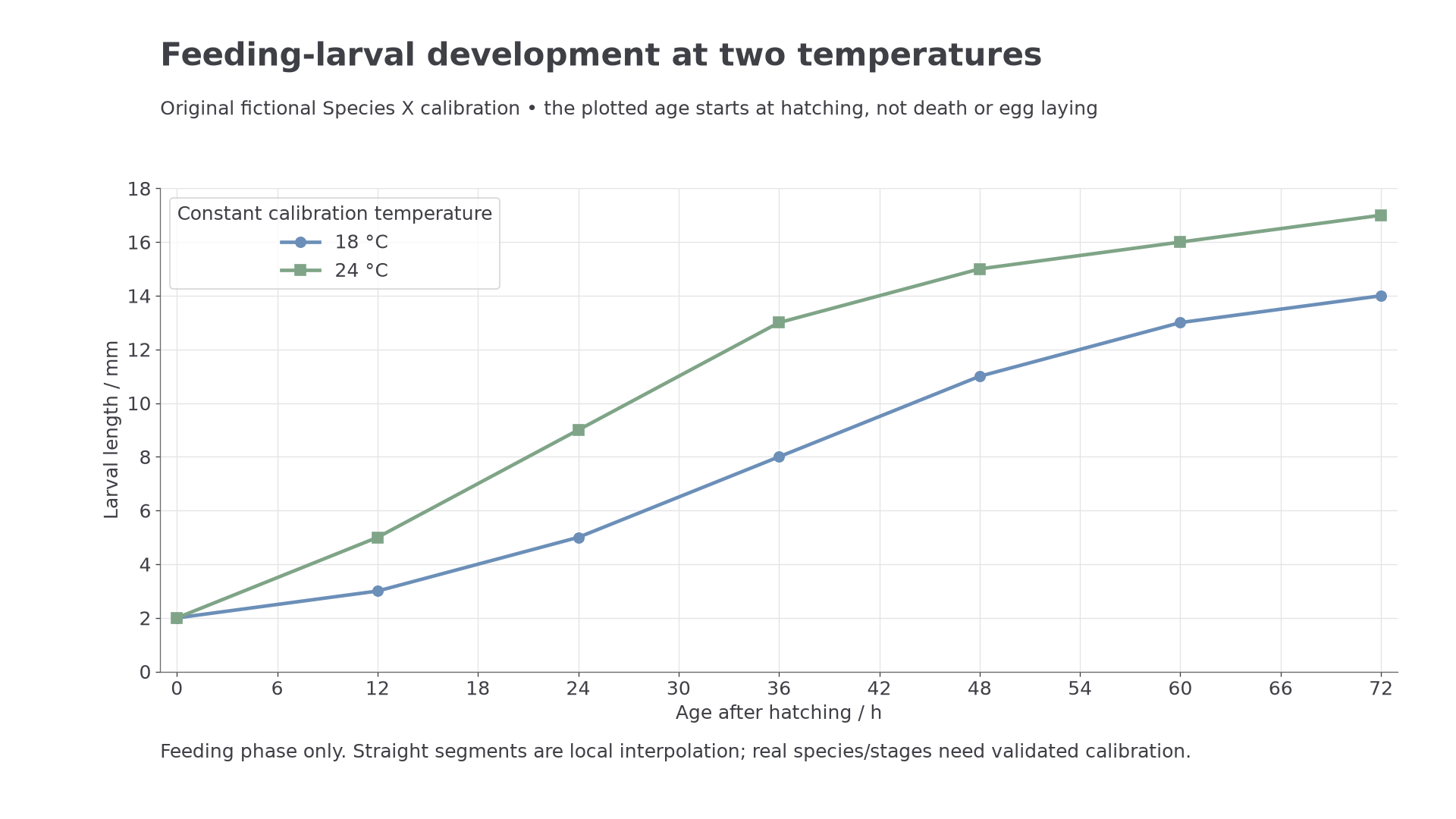
The same feeding-larval length corresponds to different ages at 18 °C and 24 °C in this original teaching calibration.
From length to an elapsed interval
A feeding larva 11 mm long corresponds to 48 h after hatching at 18 °C. At 24 °C it lies halfway between 9 mm at 24 h and 13 mm at 36 h, giving approximately 30 h. This is a plausible sense-check: the warmer calibration reaches this length sooner. Do not average the two ages if the temperature history is unknown; first establish which calibration, if either, is appropriate.
Suppose the relevant history is constant 24 °C, the larva's measured length is 11 ± 1 mm, and this fictional calibration gives an egg duration of 12–18 h. Read 10–12 mm across to the 24 °C curve and then down: the feeding-larval age is approximately 27–33 h. Add the stated egg duration to obtain 39–51 h since egg laying. This is approximately 1.6–2.1 days, using 24 h per day. These are simple bounds from the stated inputs, not a statistical confidence interval.
If the oldest evidence is represented and egg laying was after death, the lower end supports a conditional minimum of about 39 h since death. The 51 h upper end bounds this estimated time since egg laying; it does not bound how long the body might have been inaccessible before colonisation. Neither the 30 h central larval age nor the 39–51 h interval is an exact death time.
Continue this lesson.
You’re previewing NovaLearn without an account. Create a free account to read the rest.
Create free account