1.8 - Interpreting health-risk data
A larger number of deaths does not always mean a greater risk of dying: the size and composition of the population matter. This lesson shows how to compare illness and mortality data, construct useful displays, and decide what an association can establish. You will also learn how to recognise conflicting findings without choosing only the result that fits a claim.
Counts, rates and outcomes
A health comparison begins by identifying what was counted, who could have been counted, and the time period over which counting took place.
Morbidity concerns illness; mortality concerns deaths. New diagnoses and deaths are different outcomes. A study of new CVD diagnoses measures the occurrence of illness, whereas a study of CVD deaths also reflects whether people survive after developing the disease. Better treatment could reduce mortality without reducing the number of new cases. The same person may contribute to a new-diagnosis count and later to a death count, so these counts must not automatically be added together.
Incidence and prevalence
Incidence concerns new cases arising during a specified period. Prevalence is the proportion of a population that has a condition at a specified time. Existing cases belong in a prevalence count, but not in a count of first new diagnoses.
A count gives the number of events. A proportion compares that number with the relevant population. A rate additionally specifies time, such as deaths per 100,000 people per year. Read the denominator carefully: deaths among everyone in a town and deaths among people already diagnosed with CVD answer different questions. For the risk of a first diagnosis, the starting population must be free of that diagnosis.
Let be the people experiencing an outcome and the starting population at risk. For an annual mortality comparison, let be deaths during the year and the mid-year population.
For a fully followed group over a stated period:
is the risk over the stated period, expressed as a percentage.
For an annual population mortality comparison:
is annual mortality in deaths per 100,000 people per year.
The first expression estimates a probability over the whole stated period. A five-year risk is not an annual rate. If people enter or leave a study at different times, a rate may instead use their combined time under observation, called person-time; do not substitute the starting population when the supplied denominator is person-years.
A changing population
Dataset A: original NovaLearn illustrative data, not measured population statistics. The same town is recorded in two separate calendar years. The outcome is death from CVD; the populations are mid-year estimates.
| Year | CVD deaths during the year | Mid-year population |
|---|---|---|
| First year | 50 | 10,000 |
| Second year | 60 | 15,000 |
The first annual mortality rate is CVD deaths per 100,000 people per year. The second is in the same units. Deaths increased from 50 to 60, but the population grew proportionately more, so the mortality rate fell. A count alone would give the wrong direction for this comparison.
These are crude rates, calculated for the whole population without adjusting its composition. A town with more older adults may have a higher crude CVD mortality rate partly because age affects risk. Compare like outcomes, periods and population groups. An age-standardised rate adjusts age-specific rates to a common reference age distribution, making comparisons less distorted by different age structures. It is an adjusted comparison measure, not the actual number of deaths in either population.
Absolute and relative risk
An absolute risk tells you how often an outcome occurred in a group, while a relative risk compares that frequency with another group.
Dataset B: original NovaLearn illustrative cohort. Adults were classified as active or low activity at the start and followed for five years. All were initially free of diagnosed CVD; no participant was lost to follow-up. First CVD diagnoses include diagnoses in people who later died. CVD deaths are recorded separately during the same five years. These observations do not establish that activity caused the difference.
| Activity group at the start | Adults at the start | First CVD diagnoses in five years | CVD deaths in five years |
|---|---|---|---|
| Active | 10,000 | 300 | 60 |
| Low activity | 8,000 | 400 | 120 |
The active group's five-year illness risk is , compared with in the low-activity group. Their corresponding five-year risks of CVD death are and . State the outcome each time: the illness comparison and death comparison have different values. Write for the risk in the group of interest and for the risk in the named reference group, using the same units for both.
is relative risk.
is the relative percentage increase.
Subtract risks expressed as percentages to find their absolute difference in percentage points.
For illness, taking active adults as the reference gives a relative risk of , to three significant figures. The low-activity group had about 1.67 times the observed five-year risk, a relative increase of . The absolute difference was percentage points: 2 additional diagnoses per 100 adults over five years in this comparison. A 66.7% increase does not mean that 66.7% of low-activity adults developed CVD.
For CVD death, the relative risk is , the relative increase is 150%, and the absolute difference is 0.9 percentage points. A relative risk has no units. A value of 1 means equal observed risks; greater than 1 means a higher risk than the named reference group; less than 1 means a lower risk. Reversing the reference group gives the reciprocal, not a new biological finding.
Percentage change over time uses the original value as its denominator. In Dataset A, the annual mortality rate changed by : a 20% decrease. The death count changed by . Both statements are correct, but they describe different quantities.
Report the outcome, population and period alongside a risk. Give an absolute comparison as well as a relative comparison so that a large relative change is not mistaken for a large absolute probability.
These are group observations, not an exact prediction for every individual. Keep full calculator precision until the final result and use the requested rounding; do not turn a rounded relative risk into a falsely exact risk estimate.
Frequency tables and displays
The right display depends on whether the data describe categories, a distribution of measurements, or paired values for two variables.
A frequency table records how many observations belong to each category or interval. To construct one, define categories that neither overlap nor leave gaps, assign every observation once, and check that the frequencies sum to the number of observations. Include headings, units and consistent precision.
Dataset C: original NovaLearn illustrative ages at first CVD diagnosis. These 24 whole-year ages are a small sample of cases, independent of Dataset B:
31, 33, 35, 37, 39, 40, 42, 43, 44, 45, 46, 47, 49, 50, 51, 52, 54, 55, 57, 59, 61, 64, 66, 68.
| Age at diagnosis / years | Frequency / number of cases |
|---|---|
| 5 | |
| 8 | |
| 7 | |
| 4 | |
| Total | 24 |
For example, age 40 belongs in the second interval, not the first. The most frequent interval is 40 to under 50 years. This does not show that adults in that interval have the greatest CVD risk: the numbers of adults at risk in the different age groups are missing.
Bar charts and histograms
Use a bar chart for separate categories such as activity groups. For Dataset B, first calculate percentages so unequal group sizes do not mislead. Put the outcome categories on the horizontal axis, risk over five years (%) on the vertical axis, and use separate identified bars for active and low-activity adults. Start the vertical scale at zero, use equal-width bars, leave gaps between categories, and supply a key. The four heights are 3.0%, 5.0%, 0.6% and 1.5%.
Use a histogram for the frequency distribution of a continuous variable grouped into intervals. Age is continuous even when recorded to whole years. Put interval boundaries on the horizontal axis and, for these equal-width ten-year intervals, frequency on the vertical axis. Draw touching bars from 30–40, 40–50, 50–60 and 60–70 with heights 5, 8, 7 and 4. Touching bars represent adjacent intervals, rather than separate categories. With unequal interval widths, frequency density is required so that bar area represents frequency; the equal-width example does not require that calculation.
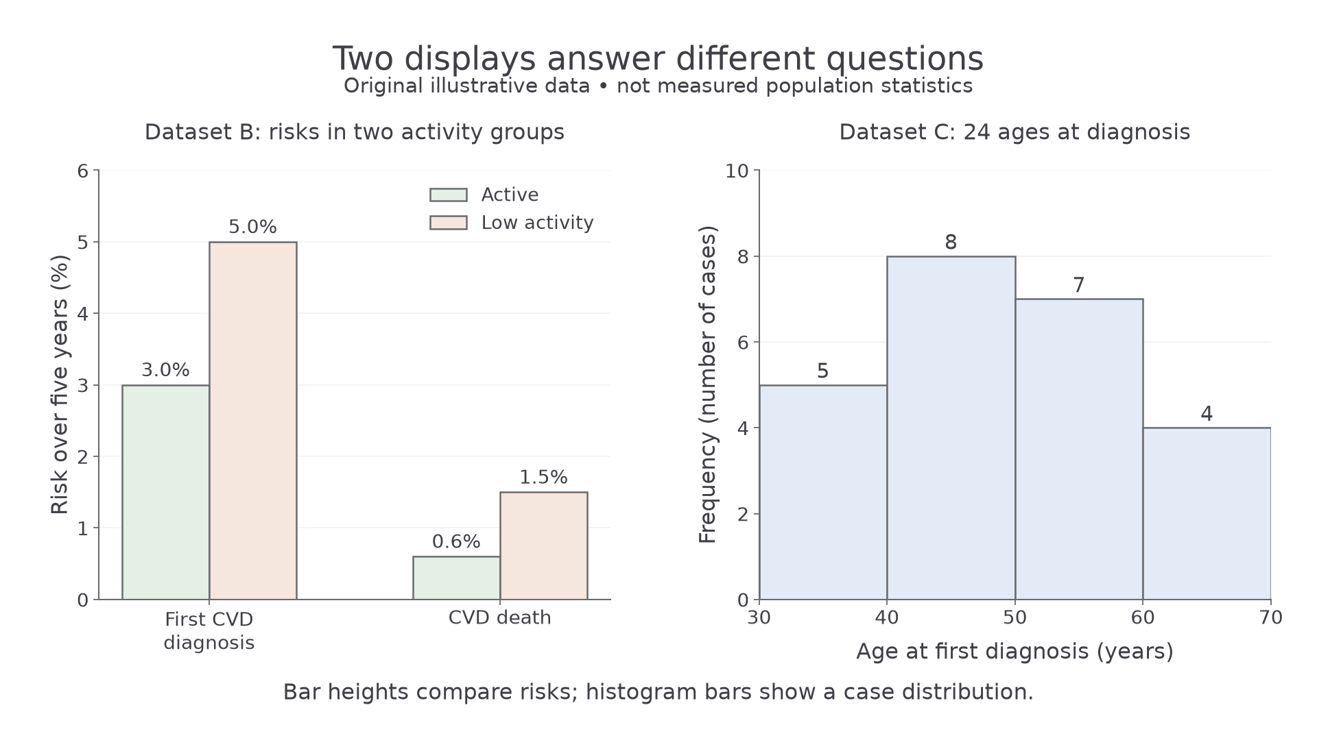
The left panel converts Dataset B counts to risks before comparing groups. The right panel represents every age in Dataset C once; its frequencies show the distribution among cases, not age-specific population risks. Both panels use zero baselines and complete axis labels.
To practise construction, draw the two panels in your notebook using the data above, then check bar heights, boundaries and labels against the figure. The construction is your drawn display; a sentence naming the trend is not evidence that you have plotted it.
Plotting paired health data
A scatter diagram displays two numerical variables measured for the same observation, with one plotted point for each pair.
Dataset D: original NovaLearn illustrative district data. Each district supplies its percentage of adults classified as inactive and its age-standardised CVD mortality rate for the same calendar year. The rates are already adjusted to the same reference age distribution. Districts are observations, not individual adults.
| District | Adults classified as inactive / % | Annual age-standardised CVD deaths per 100,000 people |
|---|---|---|
| A | 10 | 60 |
| B | 15 | 82 |
| C | 20 | 76 |
| D | 25 | 104 |
| E | 30 | 100 |
| F | 35 | 128 |
| G | 40 | 122 |
| H | 45 | 146 |
Constructing the scatter diagram
- Draw horizontal and vertical axes in your notebook or on graph paper. Put inactivity (%) on the horizontal axis and annual age-standardised CVD deaths per 100,000 on the vertical axis. In this observational comparison these are explanatory and outcome variables; calling one explanatory does not establish a causal effect.
- Use a horizontal scale from 0 to 50%, marked every 5 percentage points, and a vertical scale from 0 to 160, marked every 20. Keep the scale intervals uniform and use enough of the available plotting area to read individual points.
- Plot all eight pairs accurately. District D is at : move to 25 on the horizontal axis, then to 104 on the vertical axis. District C is ; preserve the actual value rather than moving it upwards to make a smoother trend.
- Mark points clearly and label the axes with quantities and units. Do not join successive districts as a line graph: the alphabetical order is not a time sequence.
- Compare your construction with the figure. A trend line, if used, summarises the overall pattern; it need not pass through every point. Do not delete a point simply because it weakens the trend. Investigate an unusual observation or a possible recording error first.
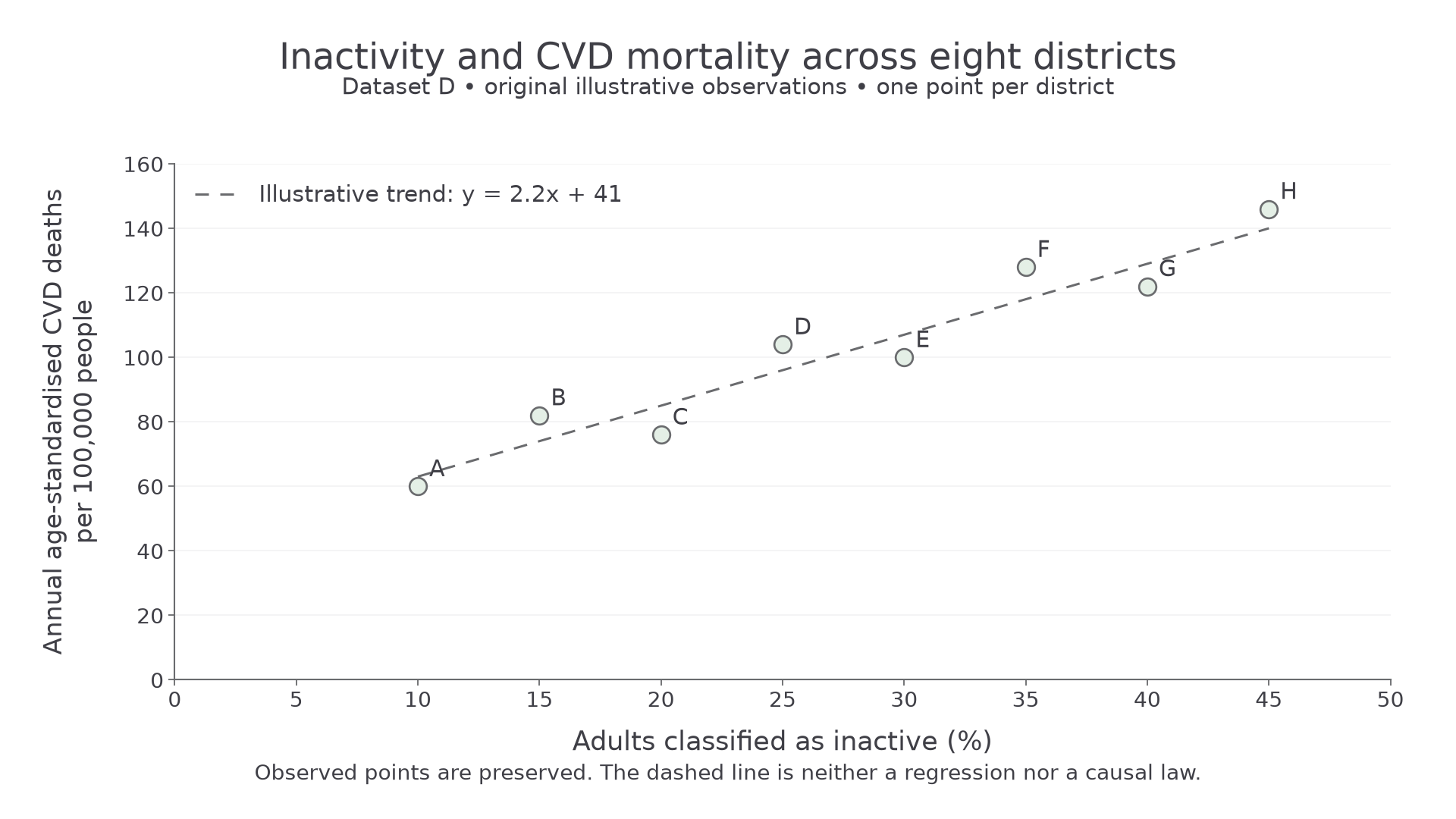
Every plotted position comes from Dataset D. The dashed line is an illustrative approximate trend, , not a calculated regression or a causal law. Here is inactivity in percentage points and is annual age-standardised CVD deaths per 100,000.
Reading the relationship
Positive correlation means that larger values of one variable tend to accompany larger values of the other. Negative correlation means that larger values tend to accompany smaller values. If no clear pattern is present, the scatter gives no clear evidence of a correlation. Strength describes how closely points follow the overall pattern; an upward trend need not be perfectly increasing between every pair of observations.
Dataset D shows a fairly strong positive association: mortality generally rises from 60 at 10% inactivity to 146 at 45%, although it falls locally from 82 to 76 between districts B and C. The scatter alone supplies no significance test. Visual strength is not proof of statistical significance or causation.
You can translate between a table, plotted coordinates and an algebraic model. Substituting into the illustrative line gives , whereas the recorded value for district E is 100. The line estimates the trend; the point records the supplied observation. Use the table or point when asked for an actual value. Estimation within the observed range is interpolation; extending beyond it is extrapolation, which is less secure because the relationship may change. This district model does not calculate an individual's chance of death.
Association and causal evidence
An association describes a pattern in observations; a causal claim says that changing one factor would change the outcome under the relevant conditions.
The positive district association could be consistent with inactivity contributing to CVD, but it does not show that inactivity produced the difference. Several explanations can fit an observational pattern.
A confounding factor is associated with both the proposed risk factor and the outcome and can distort their apparent relationship. In an unadjusted comparison, older groups may be less active and also have a higher baseline CVD risk. Age can therefore produce part of an activity–CVD association. Dataset D adjusts for age, but adjustment for one factor does not remove all possible confounding: districts may also differ in smoking, diet or access to treatment.
Reverse causation is another possibility. Illness, including disease developing before diagnosis, may reduce activity; the direction may partly be disease causing inactivity. Recording activity before a later diagnosis strengthens temporal reasoning, but does not guarantee that disease was absent when activity was recorded.
District averages also cannot establish the same relationship within individuals. The adults who are inactive need not be the adults who die from CVD. This is a limitation of drawing individual conclusions from group-level data. Conversely, a graph with little visible correlation does not prove that a factor has no causal effect: restricted ranges, other factors or inaccurate measurements can obscure a relationship.
Building a causal interpretation
Confidence increases when different kinds of evidence agree: the factor precedes the outcome; comparable studies find a consistent pattern; alternative explanations have been investigated; and a plausible biological mechanism links the factor to the disease. For example, a mechanism connecting a lifestyle factor to blood pressure or vascular damage supports a CVD interpretation, but plausibility alone does not show that this mechanism caused the observed difference.
Where safe and ethical, an intervention that changes the proposed factor and compares outcomes with a suitable control can provide stronger causal evidence than simply observing self-selected groups. It would be unacceptable to deliberately expose people to a known harmful lifestyle to obtain a disease outcome. Causal conclusions can instead draw on a body of observational, intervention and mechanistic evidence; no single pattern is an automatic proof.
An observational correlation can identify a possible risk factor. Causation requires a justified interpretation of the wider evidence, including timing, mechanisms and alternative explanations.
The numerical comparison remains useful even when its cause is uncertain. Report the observed association, then distinguish what it suggests from what the data establish.
Recognising conflicting evidence
Conflicting evidence occurs when findings support different conclusions about the same proposed relationship, so the disagreement must be examined rather than hidden.
Dataset E: complete original NovaLearn illustrative study comparison. Both studies recorded regular cycling at the start, defined as at least two cycling sessions per week, versus less than two sessions. All participants were initially free of diagnosed CVD and were followed for five years without loss to follow-up. The outcome was a first CVD diagnosis, not death. These are unadjusted observational comparisons.
| Study | Cycling group | Starting adults | First CVD diagnoses in five years | Median starting age / years |
|---|---|---|---|---|
| One | Regular | 1,000 | 60 | 65 |
| One | Less regular | 1,000 | 40 | 45 |
| Two | Regular | 2,000 | 60 | 40 |
| Two | Less regular | 2,000 | 80 | 60 |
Study One finds illness risks of 6% versus 4%, giving regular cyclists a relative risk of 1.5. Study Two finds 3% versus 4%, giving regular cyclists a relative risk of 0.75. The findings conflict in direction: one associates regular cycling with higher illness risk and the other with lower illness risk. Saying “both studies found 60 diagnoses among regular cyclists” would conceal their different denominators.
The age pattern is a plausible explanation: regular cyclists were older in Study One and younger in Study Two. Age is related to CVD risk, so these differences could contribute to the reversal. Median ages do not establish the size of the confounding effect or prove that age explains all the disagreement. Comparable age-specific or appropriately adjusted results would help separate the relationships.
Before calling findings contradictory, check whether they concern the same outcome, population, exposure definition and period. A study of CVD deaths and another of CVD diagnoses may differ because survival changed; they do not necessarily conflict about the same quantity. Among genuinely comparable studies, chance variation, measurement differences and other confounders can also contribute. A larger count is not automatically a more convincing result, and a graph without uncertainty information does not establish whether a difference is statistically significant.
A defensible conclusion from Dataset E is that these unadjusted studies give inconsistent associations, so they do not by themselves establish the causal effect of regular cycling on CVD illness. Report both results, quantify the disagreement, identify a supported possible explanation and state the limit on the conclusion. Do not average away the disagreement or select whichever study supports a preferred claim.
Reading a claim against its complete evidence
An article may report a numerical finding accurately but overstate what follows from it. Trace the headline back to the outcome, denominator and comparison, then check whether contrary results are acknowledged. The following short report is an original practice source; its values are invented for analysis, not health advice or Pearson's annual scientific article.